4.1.5. Pure Neumann boundary conditions for the Poisson equation - Using a Lagrange multiplier to remove the nullspace
First of all, in order to have only Neumann conditions, the source term \(j\) of the Poisson equation and the imposed Neumann fluxes have to fulfill a relation, which can be seen by setting the test function \(v=1\) (possible, since test functions are allowed to be arbitrary) in (4.6), which gives
If this relation is not fulfilled, the equation is not well posed. If we had a single Dirichlet condition, setting \(v=1\) is not allowed, since test functions have to vanish on the Dirichlet boundaries and this requirement is not necessary any more.
There is another complication to obtain the solution, namely the fact that the solution \(u\) is not unique: If \(u\) is a solution, \(u+c\) for any constant \(c\) is a solution as well. Any Dirichlet condition would again specify a unique constant \(c\) for which this Dirichlet condition is fulfilled, which renders the solution unique again, but in absence of any Dirichlet condition, there is an infinite number of solutions.
Both problems can be tackled simultaneously by introducing a Lagrange multiplier \(\lambda\), which fixes the spatial average of \(u\), i.e. for some prescribed \(u_\text{avg}\), we demand that the spatial average of \(u\) is \(u_\text{avg}\), i.e.
Given the fact that \(u_\text{avg}\) is a constant, we can write this as an implicit constraint
As before in Section 3.7, this constraint can be enforced by the Lagrange multiplier \(\lambda\) by minimizing
with respect to \(u\) and \(\lambda\), which gives by variation the additional weak contributions
where \(\mu\) is the test function corresponding to \(\lambda\). Therefore, we need to augment our Poisson equation from poisson_neumann.py by adding these terms to the residual as well:
from pyoomph import *
from pyoomph.expressions import *
# Load the Poisson equation for the previous class
from poisson_neumann import PoissonEquation,PoissonNeumannCondition

# Create a new Poisson equation that fixes the average with a Lagrange multiplier
class PoissonEquationWithNullspaceRemoval(PoissonEquation):
    def __init__(self,lagrange_multiplier,average_value,*,name="u",space="C2",source=0):
        # Initialize as before
        super(PoissonEquationWithNullspaceRemoval, self).__init__(name=name,source=source,space=space)
        # And store the lagrange multiplier reference
        self.lagrange_multiplier=lagrange_multiplier
        self.average_value=average_value # and the desired average value

    def define_residuals(self):
        # Add the normal Poisson residuals
        super(PoissonEquationWithNullspaceRemoval, self).define_residuals()

        # Add the contributions from the Lagrange multiplier
        l,ltest=self.lagrange_multiplier,testfunction(self.lagrange_multiplier)
        u,utest=var_and_test(self.name)
        self.add_residual(weak(u-self.average_value,ltest)+weak(l,utest))
Obviously, we load the old class PoissonEquation and inherit from it. In the define_residuals(), we first use a super call to call define_residuals() of the non-augmented PoissonEquation to add the normal residuals to the weak form. Then, the missing terms are added. However, the Lagrange multiplier \(\lambda\) is not defined yet and it cannot be defined in the PoissonEquationWithNullspaceRemoval class, since the latter will be restricted to the domain \(\Omega\). Any field definitions in the define_fields() method would hence add fields on \(\Omega\), but \(\lambda\) is just a simple real number, not a field.
Therefore, \(\lambda\) will be introduced by an own class. Since \(\lambda\) has no spatial dependence, it can be best done by using the ODEEquations class (see chapter Section 3), which allows the definition of real valued variables:
# A single "ODE", which is used as storage for the Lagrange multiplier value
class LagrangeMultiplierForPoisson(ODEEquations):
    def __init__(self,name):
        super(LagrangeMultiplierForPoisson, self).__init__()
        self.name=name

    def define_fields(self):
        self.define_ode_variable(self.name)
Note that we do not add any residuals for \(\lambda\) inside this class. The single purpose of this class is to provide the storage of a real-valued variable \(\lambda\), whereas the contributions to the residuals are entirely done in the weak form of the augmented Poisson equation.
Finally, we need to couple both parts in the definition of the problem:
class PureNeumannPoissonProblem(Problem):
    def define_problem(self):
        mesh = LineMesh(minimum=-1, size=2, N=100)
        self.add_mesh(mesh)

        # Create the Lagrange multiplier (just a single value)
        lagrange = LagrangeMultiplierForPoisson("lambda")
        lagrange += ODEFileOutput() # Output it to file as well
        self.add_equations(lagrange@"lambda_space") # And add it to a space called "lambda_space"

        l=var("lambda",domain="lambda_space") # Bind it. Important to pass the domain name here!
        # and pass it to the augmented Poisson equation
        equations = PoissonEquationWithNullspaceRemoval(l,10,source=0)
        equations += TextFileOutput() # output
        # And the Neumann conditions
        equations += PoissonNeumannCondition("u",-1) @ "left"
        equations += PoissonNeumannCondition("u",1) @ "right"
        self.add_equations(equations@"domain")


if __name__ == "__main__":
    with PureNeumannPoissonProblem() as problem:
        problem.solve()  # Solve the problem
        problem.output()  # Write output
In the define_problem() method, it is noteworthy that the LagrangeMultiplierForPoisson object is stored in another domain (named "lambda_space") than the Poisson equation. This is necessary, since the domain "domain" is already bound to the interval \(\Omega=[-1,1]\) of the line mesh. By the var() statement, we bind the just allocated variable \(\lambda\) to the local variable l and pass it together with the desired average value \(u_\text{avg}=10\) to the PoissonEquationWithNullspaceRemoval object. Thereby, both parts, the augmented Poisson equation on \(\Omega\) and the separately defined Lagrange multiplier \(\lambda\) are coupled. The remainder is as before, but now two PoissonNeumannCondition objects are created.
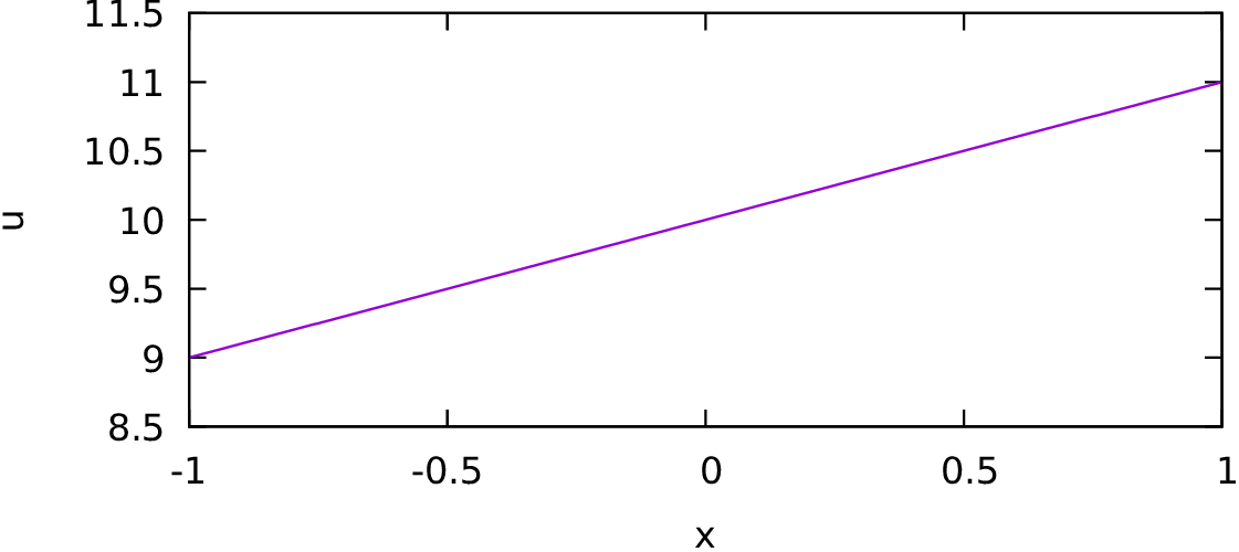
Fig. 4.4 Poisson equation with pure Neumann conditions, i.e. Neumann boundary conditions at the left and right. We have to enforce an average value (here \(10\)) to make the solution unique.
The output (plotted in Fig. 4.4) indeed shows that the average of \(u\) is \(10\) and that the value of the Lagrange multiplier \(\lambda=0\). If one instead violates the condition (4.7) by imposing an ill-posed combination of the Neumann fluxes and the source \(g\), the Lagrange multiplier will attain a non-zero value, which can be seen as follows: Let us first write down the full augmented residual form:
Upon selection \(v=1\) and \(\mu=0\) as well as \(v=0\) and \(\mu=1\), we arrive at
Obviously, the previous constraint (4.7) can now be fulfilled by solving for the correct value \(\lambda\), which introduces a new source function \(g^*=g-\lambda\), so that this constraint is fulfilled. The test space of \(\lambda\) on the other hand is used to set the average of \(u\) to \(u_\text{avg}\).