4.1.10. Changing the coordinate system
By default, the coordinate system is just the normal Cartesian one. This holds true for \(1\)d, \(2\)d and \(3\)d geometries. However, a lot of physical problems are in fact \(3\)d, but have a rotational symmetry, i.e. can be considered to be axisymmetric so that axisymmetric cylindrical coordinates can effectively reduce the problem to a computationally favorable \(2\)d problem. With a single line of code, i.e. by calling set_coordinate_system(), one can change the coordinate system from \(2\)d Cartesian to axisymmetric cylindrical coordinates:
# Load the previous code
from poisson_2d_adaptive import *


if __name__=="__main__":
    with AdaptivePoissonProblem2d() as problem:
        # Change the coordinate system to axisymmetric
        problem.set_coordinate_system(axisymmetric)
        # The rest is the same
        problem.max_refinement_level = 5
        problem.max_permitted_error = 0.0005
        problem.min_permitted_error = 0.00005
        problem.solve(spatial_adapt=problem.max_refinement_level)
        problem.output()
Note that the radial coordinate \(r\) is given by the \(x\)-direction, which can be accessed in both cases by var("coordinate_x"), whereas the \(y\)-axis becomes the coordinate along the axis of symmetry (often called \(z\) in cylindrical coordinates). In pyoomph, this coordinate is hence accessible via var("coordinate_y"). The variable var("coordinate") will expand to the vector consisting of these coordinates.
When changing the coordinate system, pyoomph will intrinsically modify the weighting in the spatial integral terms in the weak form and will evaluate the spatial derivatives accordingly.
Besides the coordinate system axisymmetric, which works in \(1\)d and \(2\)d geometries, there is also the radialsymmetric coordinate system, which works in \(1\)d geometries only. It can be used to simulate problems that have the full rotational symmetry of a sphere by just solving for the radial direction. In both cases, it is important to make sure that the geometry (i.e. the mesh) has only non-negative \(x\)-coordinates (i.e. radial coordinates). Furthermore, one cannot impose Neumann conditions at \(x=0\) (i.e. \(r=0\)), since the spatial integrals \(\int \ldots \mathrm{d}S\) will expand to \(2\pi\int \ldots r\mathrm{d}l\). Since \(r=0\), there cannot be any contribution from Neumann conditions here. However, the symmetry assumption usually requires to have a vanishing Neumann flux at \(r=0\) anyhow.
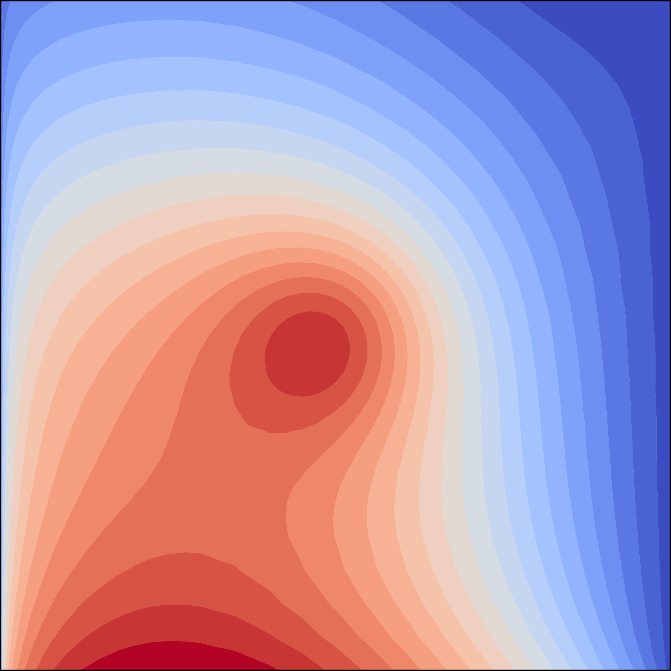
Fig. 4.8 Poisson equation with an axisymmetric coordinate system.