4.5. The Helmholtz equation with PML
Here, we consider the Helmholtz equations which arises when e.g. applying separation of variables to the wave equation. The solution of the Helmholtz equation then gives the amplitude of e.g. a periodic sound field. However, as we will see in this tutorial, boundaries will automatically reflect the wave, either by posing a node for Dirichlet conditions or an antinode for zero Neumann conditions. We will also introduce the concept of perfectly matched layers (PML), which can be used to mimick an infinite domain, i.e. where an outgoing wave just leaves the boundary without any reflection.
But let’s first start with the basis, namely the Helmholtz equation
The weak formulation is obviously analogous to the Poisson equation, but the source term is now dependent on the unknown field \(u\) as well, entering linearly with the squared wave number \(k\) as factor. Using the test function \(v\), the weak formulation reads
While this is trivial to implement with the knowledge obtained so far throughout this tutorial, it is not trivial to pose appropriate boundary conditions that allow for the wave to leave the considered domain without reflection. While this can in principle be done by solving a Dirichlet-to-Neumann problem along the boundaries, pyoomph does not allow for this. Pyoomph is a local finite element method, whereas Dirichlet-to-Neumann problems are always nonlocal and usually solved by boundary integral methods instead. In particular, the resulting Jacobian won’t be sparse (at least the boundary contributions) and the linear solvers pyoomph is using are optimized for sparse matrices only. Moreover, pyoomph just does not allow to pose nonlocal integral equations like convolution integrals.
The alternative are the perfectly matched layers (PML), which can be written as local contribution. However, this comes at some expenses: Firstly, the domain has to be extended by a PML regions and secondly, the real Helmholtz equation must be generalized to complex values. Once this is done, a complex coordinate transformation according to
with complex spatially dependent functions \(\gamma_i(\vec{x})\) can be utilized to alter the oscillatory behavior of the wave to an increasingly damped wave which vanishes once it reaches the end of the PML region. Obviously, when \(\gamma_i=1\), the equation behaves like the conventional Helmholtz equation, so the complex coordinate transformation with \(\gamma_i(\vec{x})\neq 1\) is only applied in the PML regions, not in the region of interest. If the wave leaves the domain of interest through a boundary in \(x\)-direction, we therefore set
where \(\sigma_x(x)\) is an inverse distance to the exterior boundary of the PML region, e.g. \(\sigma_x=|X_\mathrm{PML}-x|^{-1}\), where \(X_\mathrm{PML}\) is the \(x\)-position of the PML exterior boundary. For this particular case, we keep \(\gamma_y=1\), where it is vice versa for wave leaving the domain of interest in \(y\)-direction. If the wave leave the domain through a corner, both tranformations are active. We introduce a complex unknown field \(U(\vec{x})\) by the splitting \(U=u+iu_\mathrm{Im}\) with corresponding complex test function \(V=v+iv_\mathrm{Im}\) and generalize the Helmholtz equation (for the 2d Cartesian case) to
here, \(\mathbf{T}=\mathrm{diag}(\gamma_y/\gamma_x,\gamma_x/\gamma_y)\) applies the necessary transformation of the differential operators. Thereby, in the PML regions, the waves get exponentially damped but are still coupled with the surroundings, i.e. thereby still accounting for the coupling which leads to a nonlocal Dirichlet-to-Neumann problem.
To make all these aspects more clear, let’s just implement a circular hole in a rectangular domain and solve the Helmholtz equation with a prescribed Dirichlet value on the circle boundary. We will add an option to activate or deactivate the PML to see the effect. We skip the mesh class here for brevity. It is quite some work if you want to add the individual PML regions. However, the mesh class is of course part of the example code file.
Our Helmholtz equation now takes, besides the wavenumber \(k\), the potential scalings \(\gamma_x\) and \(\gamma_y\):
class HelmholtzEquation(Equations):
    def __init__(self, k,gamma_x=1, gamma_y=1):
        super().__init__()
        self.k = k # wavenumber
        self.gamma_x = gamma_x # PML complex coordinate transformation coefficient in x-direction
        self.gamma_y = gamma_y # PML complex coordinate transformation coefficient in y-direction

    def has_PML(self):
        # Check if PML is used, i.e., if the gamma_x or gamma_y are not equal to 1
        return self.gamma_x != 1 or self.gamma_y != 1

    def define_fields(self):
        # Define the scalar fields for the Helmholtz equation
        self.define_scalar_field('u', 'C2')
        if self.has_PML():
            # If PML is used, define an additional scalar field for the imaginary part
            self.define_scalar_field('u_Im', 'C2')

    def define_residuals(self):
        u,v=var_and_test("u")
        if not self.has_PML():
            # Standard Helmholtz equation without PML
            self.add_weak(grad(u),grad(v)).add_weak(-self.k**2 * u, v)
        else:
            # Helmholtz equation with PML, only works for 2D Cartesian coordinates like here
            if self.get_nodal_dimension()!=2 or self.get_coordinate_system().get_id_name() != "Cartesian":
                raise ValueError("PML Helmholtz equations only implemented for Cartesian 2D problems")

            uIm,vIm=var_and_test("u_Im")
            # complex field and test function
            U,V=u+imaginary_i()*uIm,v+imaginary_i()*vIm
            # scaled gradient
            mygrad=lambda f: vector(self.gamma_y/self.gamma_x*grad(f)[0], self.gamma_x/self.gamma_y*grad(f)[1])
            # complex weak form
            R=weak(mygrad(U),grad(V))-weak(self.k**2 * U, V*self.gamma_x*self.gamma_y)
            # add real and imaginary parts separately
            self.add_residual(real_part(R)+imag_part(R))
If no scaling is set, the function has_PML will return False and we only define a real-valued field u with the conventional weak form of the Helmholz equation. Otherwise, we also add a field for the imaginary part of \(U\) and define the weak form of the PML-modified Helmholtz equation instead. Note how we can access the imaginary unit by imaginary_i(). This allows us to assemble the complex-valued field \(U\) by adding the real and imaginary part. Since pyoomph only handles real-valued residuals, we have to cast it back to a real-valued residual by applying real_part() and imag_part() on it. Again, since the test functions of the real and imaginary part can be chosen arbitarily, the superposition of both residuals is sufficient in the add_residual() call.
As usual, the problem class just defines some reasonable parameters in the constructor. We also add a flag here whether we want to consider the PML part or not. If we have PML activated, we first must set up the expressions for \(\gamma_x\) and \(\gamma_y\), which depend on the distances to the exterior PML boundaries. In order to activate the coordinate transformation only in the PML regions, we introduce two helper fields, "PML_indicator_x" and "PML_indicator_y". These are D0 fields, i.e. having a constant value within each element. By combining it with a DirichletBC without any boundary restriction, the values of these indicator fields will be set without having to solve for additional unknowns. By the indicator fields, we can blend in the PML coordinate transformation where necessary. Also note that we set \(U=0\) at the exterior boundary of the PML region and suppress the imaginary part at the circle, where we prescribe the Dirichlet condition for \(u\).
class HelmholtzProblem(Problem):
    def __init__(self):
        super().__init__()
        self.k = square_root(50) # wavenumber
        self.a=0.2 # radius of the circle
        self.L=2 # half the side length of the square domain
        self.use_PML=True # use PML or not
        self.N_PML=5 # number of nodes in the PML region
        self.d_PML=0.2 # thickness of the PML region
        self.mesh_coeff_PML=1 # node placement coefficient for the PML region

    def define_problem(self):
        self+=RectangularMeshWithHoleAndPMLBoundary()

        if self.use_PML:
            x,y=var(["coordinate_x","coordinate_y"])
            # Inverse PML distance coefficients. Diverge at the far boundary
            sigma_x=subexpression(maximum(1/((self.L+self.d_PML)-x),1/((self.L+self.d_PML)+x)))
            sigma_y=subexpression(maximum(1/((self.L+self.d_PML)-y),1/((self.L+self.d_PML)+y)))
            # PML complex coordinate transformations, only active in the PML region by the indicator functions
            gamma_x=1+var("PML_indicator_x")*imaginary_i()/self.k*sigma_x
            gamma_y=1+var("PML_indicator_y")*imaginary_i()/self.k*sigma_y
            # Indicator functions for PML, elementally constant, set to 1 in PML region, 0 in physical domain
            pml_eqs=ScalarField("PML_indicator_x", "D0")+DirichletBC(PML_indicator_x=(heaviside(absolute(x)-self.L)))
            pml_eqs+=ScalarField("PML_indicator_y", "D0")+DirichletBC(PML_indicator_y=(heaviside(absolute(y)-self.L)))
            pml_eqs+=DirichletBC(u_Im=0)@"circle"
            pml_eqs+=DirichletBC(u=0,u_Im=0)@"PML_outer"
        else:
            pml_eqs=0 # No PML equations if not used
            gamma_x, gamma_y=1, 1 # No PML scaling factors if not used

        eqs=HelmholtzEquation(self.k,gamma_x,gamma_y)
        eqs+=MeshFileOutput()
        eqs+=DirichletBC(u=0.1)@"circle"
        eqs+=pml_eqs # Add PML equations if used

        self+=eqs@"domain"
The run code is again trivial:
with HelmholtzProblem() as problem:
    problem.solve()
    problem.output()
The results are depicted in Fig. 4.23 and speak for themselves. Indeed the radial symmetry of the wave without any reflection on the boundaries can be achieved by PML.
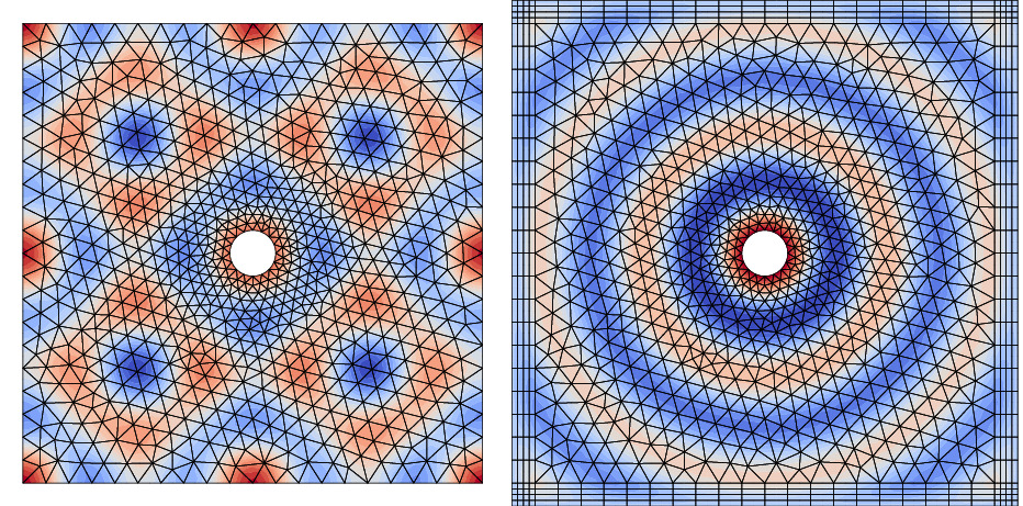
Fig. 4.23 (left) Solution with zero Neumann conditions and (right) with PML.
Note
This example is a direct adaption of the case discussed in oomph-lib here: https://oomph-lib.github.io/oomph-lib/doc/pml_helmholtz/scattering/scattering.pdf