4.1.2. One-dimensional Poisson equation with Dirichlet boundary conditions
Let us first consider the Poisson equation on a simple interval, i.e. on the domain \(\Omega=[-1,1]\). Furthermore, we initially restrict to impose Dirichlet boundary conditions \(u=0\) at \(x=-1\) and \(x=1\). The source function is simply \(g=1\). If there are no Neumann conditions, the weak formulation (4.6) reduces to
This weak form is implemented in a Equations class as follows:
from pyoomph import *
from pyoomph.expressions import *  # Import grad & weak


class PoissonEquation(Equations):
    def __init__(self, *, name="u", space="C2", source=0):
        super(PoissonEquation, self).__init__()
        self.name = name  # store the variable name
        self.space = space  # the finite element space
        self.source = source  # and the source function g

    def define_fields(self):
        self.define_scalar_field(self.name, self.space)  # define the unknown scalar field

    def define_residuals(self):
        u, v = var_and_test(self.name)  # get the unknown field and the corresponding test function
        # weak formulation in residual form: (grad(u),grad(v))-(g,v)
        residual = weak(grad(u), grad(v)) - weak(self.source, v)
        self.add_residual(residual)  # add it to the residual
We define a new class PoissonEquation, inherited from the Equations class. In the constructor, we can pass the source function \(g\), a name of the unknown field \(u\) (defaults to "u") and a finite element space, which defaults to "C2". More on finite element spaces will be discussed later on in Section 4.2. The passed arguments are stored in the object.
In the define_fields() method, we use define_scalar_field() to create a field with the desired name self.name on the finite element space self.space. Finally, in the method define_residuals(), the residual form is defined. To that end, we first bind the local variables u and v to the unknown field \(u\) and the corresponding test function \(v\). The shorthand notations \((\ldots,\ldots)\) for the spatial integrals (cf. (4.5)) are written in python via the function weak(). The gradients of both the unknown field \(u\) and the test function \(v\) are obtained grad(), i.e. by grad(u) and grad(v), respectively. The weak form in residual formulation, stored in the local variable residual is eventually added by the method add_residual(), which completes the definition of the weak form of the PoissonEquation.
To actually use this equation, we again have to write a problem class, inherited from the generic Problem class:
class PoissonProblem(Problem):
    def define_problem(self):
        mesh = LineMesh(minimum=-1, size=2, N=100)  # Line mesh from [-1:1] with 100 elements
        # Add the mesh (default name is "domain" with boundaries "left" and "right")
        self.add_mesh(mesh)

        # Assemble the system
        equations = PoissonEquation(source=1)  # create a Poisson equation with source g=1
        equations += DirichletBC(u=0) @ "left"  # Dirichlet condition u=0 on the left boundary
        equations += DirichletBC(u=0) @ "right"  # and u=0 on the right boundary
        equations += TextFileOutput()  # Add a simple text file output
        self.add_equations(equations @ "domain")  # Add the equation system on the domain named "domain"
Again, the work is done in the define_problem() method. First of all, we need to define the geometry where the equation should be solved. Geometries in pyoomph are always defined via mesh templates. A mesh template provides spatially discretized geometric domains with named boundaries. The simplest mesh template is the LineMesh, which is just an interval subdivided into \(N\) elements. To create the desired domain \(\Omega=[-1,1]\), we pass the keyword arguments minimum=-1 and size=2 and divide it into N=100 elements. This mesh template is added to the problem with the add_mesh() method. A mesh template has named domains and boundaries. The default names for the LineMesh are "domain" for the domain, i.e. here \([-1,1]\), "left" for the left boundary, i.e. \(x=-1\) and "right" for the right boundary, here \(x=1\).
Then, the equation system is assembled. We create the previously implemented equation class PoissonEquation, setting the source function \(g\) to \(1\). We then add DirichletBC objects and use the @ operator to restrict these Dirichlet conditions to the boundaries "left" and "right". Also a TextFileOutput is added to the equation system to provide output as a simple text file. Finally, the entire system stored in Equations is added to the problem via add_equations(). Note that we have to restrict the equations once more to the desired domain "domain" which is provided by the previously added mesh template, i.e. the added LineMesh.
Finally, we just have to create the problem, solve it and write the output via
if __name__ == "__main__":
    with PoissonProblem() as problem:
        problem.solve()  # Solve the problem
        problem.output()  # Write output
Opposed to the ODEs in the previous chapter, there is no need for a temporal integration, i.e. the run() method of the problem is not required, but instead we use solve(). We also have to manually call the output() method to write the output to file, which is plotted in Fig. 4.1.
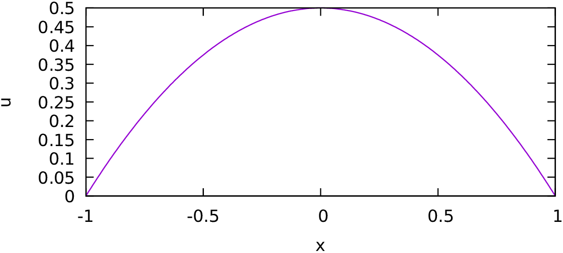
Fig. 4.1 One-dimensional Poisson equation with Dirichlet boundaries.