3.11.9. Lyapunov exponents
After a stationary state becomes unstable due to bifurcations, it can either converge to another stationary solution, diverge or show nontrivial temporal dynamics. In the latter case, the dynamics can be either periodic, quasi-periodic or chaotic. A prominent example of chaotic dynamics is given by the Lorenz system, which was already discussed in Section 3.6.5. However, just from the trajectory of the system alone, it is not directly apparent that it is indeed a chaotic system.
A necessary requirement for deterministic chaos is the sensitivity to small changes of the initial conditions. If a system is chaotic, a small perturbation in the initial condition will grow over time and the long term dynamics of the unperturbed and the perturbed system will be separated by a growing distance in phase space. However, usually, dissipative systems are considered, i.e. systems that relax on a strange attractor, which is bounded in phase space. Therefore, eventually both the unperturbed and perturbed trajectories can converge to the same strange attractor and the distance between both trajectories in time will be bounded as well.
Therefore, instead of measuring the divergence of perturbations in the initial conditions (which is ultimately bounded) it is beneficial to investigate the growth of a tiny perturbation along the trajectory. Let \(\vec{x}(t)\) be a trajectory, then we are interested in how a perturbation \(\vec{x}(t)+\delta\vec{x}(t)\) will develop. Here, we choose a tiny initial perturbation vector \(\delta\vec{x}(0)\) and make sure that it remains tiny during its evolution, so that the linear dynamics around \(\vec{x}(t)\) alone govern the choice of \(\delta\vec{x}(0)\). This can be achieved by either choosing the magnitude of the initial perturbation \(\delta\vec{x}(0)\) sufficiently small that it does not grow within the considered simulation time to a magnitude where nonlinear contributions become relevant. Alternatively, one can renormalize \(\delta\vec{x}(t)\), e.g. after each \(n^\text{th}\) time step, to a tiny magnitude, while monitoring its exponential growth.
More precisely, for a system \(\partial_t\vec{x}=\vec{F}(\vec{x})\), it is sufficient to calculate the linearized evolution of
where \(\mathbf{J}\) is the linearization of \(\vec{F}\), i.e. the Jacobian along the trajectory. Due to nonlinearities, the Jacobian is not constant along the trajectory, but the long term dynamics still follow an exponential growth or decay in the long-term limit, i.e. \(\delta\vec{x}(t)\sim\exp(\lambda t)\). For an \(N\)-dimensional system, we generically have \(N\) different solutions for the exponent \(\lambda\), which are called Lyapunov exponents. If at least one \(\lambda\) is positive, a random perturbation will generically grow over time. If the sum of all Lyapunov exponents is additionally negative, we converge to a strange attractor, i.e. an indicator for chaos. Note that one Lyapunov exponent is usually zero (if the solution is not attaining a stationary solution), corresponding to the initial perturbation \(\delta\vec{x}(0)\propto\partial_t\vec{x}(0)\), i.e. just a shift in the direction of the trajectory \(\vec{x}(0)\).
Conventional implementations to numerically calculate Lyapunov exponents rely on the explicit form (3.17). However, not all systems can be written in this form, e.g. the pendulum constraint in Section 3.7, which has no time derivative. Since pyoomph allows us to formulate equations in the implicit residual formulation \(\vec{R}(\partial_t\vec{x},\vec{x})=0\), a general form of (3.17) reads
with the mass matrix \(\mathbf{M}\) and the Jacobian (without any time-derivatives) \(\mathbf{J}\).
Warning
This form is of course only valid if the maximum time derivative order is one, i.e. for second order time derivatives, again the usual substitution has to be done, cf. Section 3.6.4.
To calculate Lyapunov exponents, pyoomph comes with the class LyapunovExponentCalculator from the pyoomph.utils.lyapunov module. It starts with one or multiple initially random guesses of \(\delta\vec{x}(0)\) and integrates (3.18) along the trajectory. If more than one guess is taken, a Gram-Schmidt orthogonalization is performed after each step. Thereby, components of the faster growing perturbations (i.e. corresponding to higher Lyapunov exponents \(\lambda\)) are removed from the slower growing or even decaying perturbation components. Automatically, the class LyapunovExponentCalculator writes the desired number of Lyapunov exponents \(\lambda\) to a text file. Due to the random initial guess, usually the largest Lyapunov exponents will be calculated, but these are normally also the most interesting ones. Moreover, the class LyapunovExponentCalculator allows to select two times, \(T_\text{wait}\) and \(T_\text{relax}\), by the keyword arguments waiting_time and prerelaxation_time. The former is the time delay when the actual calculation of the perturbation vector sets in; the latter is the time offset to start the actual calculation of the Lyapunov exponents, i.e. allowing some time to let the perturbation vectors adjust according to the dynamics. The Lyapunov exponents will then be estimated by
where \(T_0=T_\text{wait}+T_\text{relax}\).
As an example, we will check the Lorenz system (with the default parameters \(\sigma=10\), \(\rho=28\) and \(\beta=8/3\)) from Section 3.6.5 for chaos in the following. When modifying the run code of section Section 3.6.5 to
    # Import the LyapunovExponentCalculator from the utils module
    from pyoomph.utils.lyapunov import LyapunovExponentCalculator

    with LorenzProblem() as problem:
        # We want to save memory, since we have a fine temporal discretization.
        # So we do not write state files for continue simulations
        problem.write_states=False
        # Add the LyapunovExponentCalculator to the problem.
        # Calculating k=3 Lyapunov exponents. Starting after t=10, then relaxing perturbation vectors until t=10+5
        # Then start the actual Lyapunov exponent calculation
        problem+=LyapunovExponentCalculator(k=3,waiting_time=10,prerelaxation_time=10,store_as_eigenvectors=False,use_crank_nicholson_integration=False)
        # Run it with a rather fine time step
        problem.run(endtime=200,outstep=0.001)
we get a file called lyapunov.txt in the output directory. The delay times are chosen to \(T_\text{wait}=T_\text{relax}=10\). The resulting plot is the following, where we also added the long-time limit literature values by dotted lines. The sum of all Lyapunov exponents corresponds to the phase space divergence, i.e. the trace of the Jacobian, which can be obtained analytically by \(\sum_{i=1}^3 \lambda_i=-\sigma-1-\beta\approx -13.666\). Finer time steps give even better agreement.
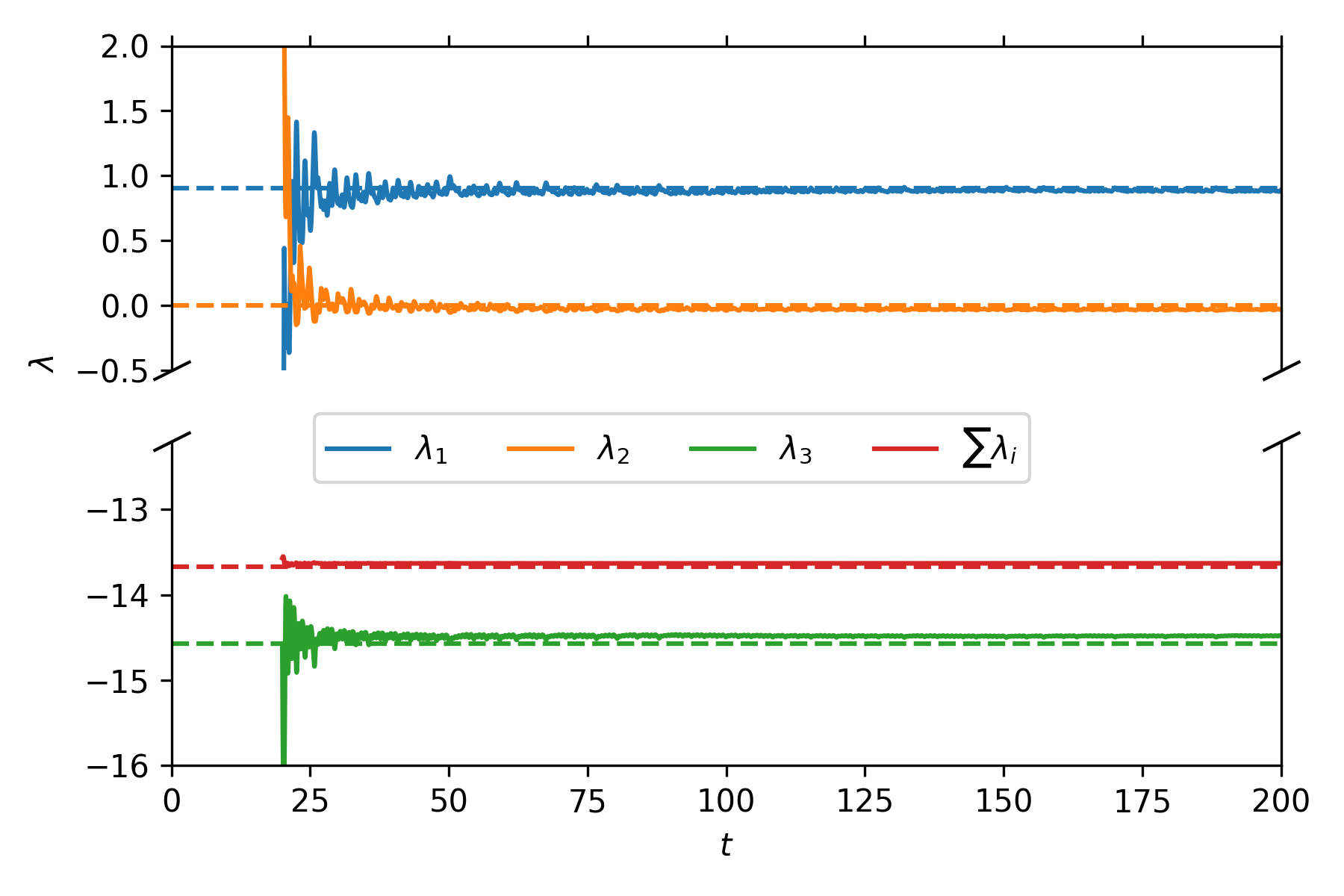
Fig. 3.16 Lyapunov spectrum of the Lorenz system with \(\sigma=10\), \(\rho=28\) and \(\beta=8/3\). Dotted lines are the long-time limit literature values.
As expected, we have one positive Lyapunov exponent (indicating chaos), one around zero (in the direction of the trajectory), and another one negative, so that the sum of all is in total negative (requirement for phase volume contraction, i.e. for a strange attractor).
The method described here can also be applied to spatio-temporal PDEs, which are discussed later in Section 5.