3.11.8. Deflated solving and deflated continuation
Nonlinear problems generically have multiple solutions for fixed parameter values. While for the pitchfork normal form (3.16), all solutions can be found analytically (depending on the parameter either 1 or 3 solutions), this is in general not possible, e.g. when having a sufficiently complicated system of nonlinear equations. Even numerically, it is generically not possible to be sure that you have found all solutions, in particular for automatic methods. Without any knowledge of the residuals of a system with only a single unknown, you would have to sample all potential starting guesses, from \(-\infty\) to \(\infty\), and perform Newton’s method with these initial guesses and record all found solutions.
This is of course not feasible and we therefore can only hope that any numerical algorithm can find a subset of solutions. Since a single initial guess will always run into the same solution during Newton’s method (convergence provided), we either can use multiple starting guesses (as described above), or somehow prevent that Newton’s method can run into the same solution again. This is obviously possible if we ensure that (i) all found solutions are penalized so that Newton’s method cannot converge into them and (ii) that all not yet found solutions of the original problem are still solutions of the penalized problem. These observations suggest a product of a penalizer (called a deflation operator) and the original residuals. Here, we follow the approach of Ref. [21]. If a single solution \(\vec{U}_1\) is known, we define the deflation operator
If multiple solutions \(\vec{U}_1,\vec{U}_2,\ldots,\vec{U}_n\) are known, we can just use the product of the deflation operators. This defines new residuals
which obviously fulfill the required properties. The shift \(\alpha\) prevents numerically diverging unknowns \(\vec{U}\) from being considered as a new solution, since the inverse norm can easily fall below the accuracy threshold of the Newton solver applied to \(\vec{R}_\mathrm{defl}\).
pyoomph can apply the method of Ref. [21] automatically and iterate over multiple found solutions at a given parameter value. As an example, we will calculate the solutions of a pitchfork bifurcation at a specific parameter, where three solutions exist. The considered pitchfork normal form is the same as in (3.16), so we do not reiterate it here. Also, we do not define a problem class, but assemble our problem directly in the run script:
    # Simple problems can be assembled without a specific class
    problem=Problem()
    problem+=PitchForkNormalForm(r=1,sign=-1)@"pitchfork"
    # Find the solutions by deflation
    solutions=[]
    for sol in problem.iterate_over_multiple_solutions_by_deflation(deflation_alpha=0.1,deflation_p=2,perturbation_amplitude=0.1,num_random_tries=2):
        solutions.append(sol)
    print("Found solutions at r=1 are x = ",solutions)
When running, the method iterate_over_multiple_solutions_by_deflation() will first solve the problem normally, without any deflation. The for-loop will receive the corresponding degrees of freedom. After that, the first solution is removed by the deflation operator specified above. Here, you can select the exponent \(p\) and the shift \(\alpha\) by the keyword arguments deflation_p and deflation_alpha. However, we must perturb the first solution before trying to find the next one. Otherwise, we would divide by zero. This is done by a random perturbation of the solution with an amplitude given by perturbation_amplitude. A single random try may not be enough, so we also allow specifying the number of attempted solves with different random perturbations of the previous solution, which can be selected by num_random_tries. Optionally, you can also perform a perturbation by the dominant eigenvector when adding the argument use_eigenperturbation=True. An attempted solve with the perturbation in eigendirection will then be done additionally to the random perturbation(s). Whenever a new solution is found, also this solution is considered in the deflation operator. Afterwards, all found solutions are perturbed again and new attempts are started to find even more solutions.
Depending on the generated random numbers, one either finds all three solutions \(x=0\), \(x=\pm 1\), or only two of them. Hence, deflation provides no guarantee that indeed all solutions are found, but it is at least a promising approach to find further solutions.
Deflation can furthermore be combined with parameter scanning, in a sort of continuation. Opposed to arclength continuation, we do not solve along the arclength of a single solution branch, but just scan over the parameter branch once. But at each scanned parameter value, we try to find new solutions by deflation and try to connect the solutions at the previous parameter value to the new solutions. This algorithm has been proposed in Ref. [20], which can be invoked using the method deflated_continuation():
    problem=Problem()
    r=problem.define_global_parameter(r=-1)
    problem+=PitchForkNormalForm(r=r,sign=-1)@"pitchfork"

    # Storage for the output files: Branch index -> output file
    output_files={}

    # Scan r from -1 to 1, apply deflated continuation
    for branch_index,rvalue,sol in problem.deflated_continuation(r=numpy.linspace(-1,1,50)):
        # we get the branch_index (increasing), the value of the parameter and the degrees of freedom
        if branch_index not in output_files:
            # Create an output file for the new branch
            output_files[branch_index]=problem.create_text_file_output("branch_{:02d}.txt".format(branch_index))
        # We can e.g. solve eigenproblems, or output solutions here
        problem.solve_eigenproblem(1)
        Re_ev=numpy.real(problem.get_last_eigenvalues()[0])
        # Write the output
        output_files[branch_index].add_row(rvalue,sol[0],Re_ev)
A call of deflated_continuation() expects a parameter sampling range and has similar additional optional arguments as iterate_over_multiple_solutions_by_deflation(). At each solution, the for-loop receives an increasing branch index, the current parameter value and the degrees of freedom of the solution. Feel free to calculate e.g. eigenvalues or call e.g. output() inside the loop to process the current solution. You could also consider adding a write_state() whenever a new branch index starts. With another script, you can load these states via load_state() and e.g. finalize the bifurcation diagram by arclength continuation of all found solutions.
We can indeed recover the diagram of the pitchfork normal form (cf. Fig. 3.15), however, deflated continuation cannot connect the branching points nicely. It also does not note that branch 1 and branch 2 actually belong to the same branch, if we define a branch in a result of an arclength continuation:
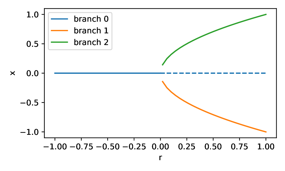
Fig. 3.15 Pitchfork solutions by deflated continuation.