3.1. Nondimensional harmonic oscillator
A simple but yet illustrative example is a harmonic oscillator (without any physical units).
3.1.1. Mathematical Formulation
Let us start with the harmonic oscillator equation for a non-dimensional unknown \(y(t)\) as function of a non-dimensional time \(t\), i.e.
with \(\omega=1\) and with the initial condition \(y(0)=1\) and \((\partial_t y)(0)=\dot y (0)=-1\).
Note
Note that we use \(\partial_t\) here instead of \(\mathrm{d}/\mathrm{d}t\) as notation for the time derivative, since we will later turn to spatio-temporal equations and in both cases, the time derivative in pyoomph is obtained by the function partial_t().
3.1.2. Python code using the predefined harmonic oscillator equation class
For the Python code, we first have to import pyoomph:
# Import pyoomph
from pyoomph import *
# Also import the predefined harmonic oscillator equation
from pyoomph.equations.harmonic_oscillator import HarmonicOscillator
Every problem you want to solve in pyoomph has to be defined in a class inherited from the generic Problem class. In the constructor of this class, i.e. the method __init__(), one should set the default parameters, e.g. here \(\omega=1\). Later on, we can change this parameter before running the simulation, but some default value has to be set. However, before doing so, we first have to call the constructor of the generic problem class, which can be done by a super() call:
# Create a specific problem class to solve your problem. It is inherited from the generic problem class 'Problem'
class HarmonicOscillatorProblem(Problem):

	# In the constructor of the problem, we can set some default values. here omega
	def __init__(self):
		super(HarmonicOscillatorProblem,self).__init__() #we have to call the constructor of the parent class
		self.omega=1 #Set the default value of omega to 1
The next important step is the definition of the problem. In our case, we have three ingredients:
We want to solve a harmonic oscillator,
with \(y(0)=1\) and \(\dot y(0)=-1\) as initial condition
and finally, we also want to get some output, namely the curve of \(y(t)\).
pyoomph takes here the approach, that all these elements can be combined by the operator +. We therefore overload the method define_problem() of the Problem class as follows:
	# The method define_problem will define the entire problem you want to solve. Here, it is quite simple...
	def define_problem(self):
		eqs=HarmonicOscillator(omega=self.omega,name="y") #Create the equation, passing omega
		eqs+=InitialCondition(y=1-var("time")) #We can set both initial conditions for y and y' simultaneously
		eqs+=ODEFileOutput() #Add an output of the ODE to a file
		self.add_equations(eqs@"harmonic_oscillator") #And finally, add this combined set to the problem with the name "harmonic_oscillator"
Let us go through these steps once more: The function define_problem() will be called, whenever we try to run the simulation with our problem class HarmonicOscillatorProblem. Within this method, we first create an instance of the HarmonicOscillator equations (which will be re-implemented by hand in the next section). There, we pass omega (\(=\omega\)) from the problem to the equation class and inform the equation class that the unknown variable of the harmonic oscillator shall be called \(y\).
In the next step, this equation is augmented with an instance of InitialCondition, setting the initial condition of \(y(t)\) to \(y(t)=1-t\). Here, we use the function var() with the argument "time" to obtain the time variable \(t\) and combine it into an expression 1-var("time"), i.e. \(1-t\). However, above we stated that the initial condition shall be \(y(0)=1\) and \(\dot{y}(0)=-1\). But in fact, if one evaluates \(1-t\) and its temporal derivative at \(t=0\), one indeed recovers these initial conditions. Hence, this trick allows one to express the required two initial conditions by a single statement. Even more, one can e.g. set the initial condition from a known analytical solution, e.g. via InitialCondition(y=A*cos(self.omega*var("time")+phi)) for some amplitude A and phase phi.
Finally, all simulations are meaningless if there is no output. Therefore, an instance of the output class ODEFileOutput is added to the combined object of HarmonicOscillator+InitialCondition. This object will make sure that output of the ODE is written to a file.
At this stage, the combined object of the harmonic oscillator ODE, the initial condition and the output object are just stored in the local variable eqs, i.e. the problem class does not know yet that we want to solve this. This is done by adding the combined equation object to the problem by the method add_equations(). However, before doing so, the equations have to be restricted to a particular named domain. For ODEs, this domain name is quite arbitrary, but for multi-physics, the domain name identifies the spatial domain where the equations shall be solved, e.g. in either the gas or the liquid phase in multi-phase problems. To restrict equations to a domain, the operator @ is used, followed by the desired domain name. For the case of the ODE here, the domain name ("harmonic_oscillator" here), will just influence the name of the output file.
The only step remaining at this stage is running the simulation:
if __name__=="__main__":
	with HarmonicOscillatorProblem() as problem:
		problem.run(endtime=100,numouts=1000)
Here, it is first checked whether the current script is the main script, a typical step in Python scripts to allow for the import of definitions in external scripts without invoking any code execution. In the next step, an instance of the problem is created and finally, the simulation is started and solved until \(t=100\) using the method run(). The number of (here equidistant) output steps is set to 1000, i.e. an output interval of \(\Delta t_\text{out}=0.1\).
To run the script, just invoke Python on it, either via a command line or via a Python IDE.
By default, the output will be written to a sub-directory of the current directory with the name of the executed script, but without the extension .py. If the script is called nondim_harmonic_osci.py, the output can be found in the sub-directory nondim_harmonic_osci/. Here, multiple files can be found. In the sub-folder _ccode, we can find the generated C code of the equations. The sub-directory _states contains state files, which allow one to continue a previously interrupted simulation (cf. Section 5.5 later on). Since we have added an ODEFileOutput object to our equations (defined on the domain "harmonic_oscillator"), we will also find a text file harmonic_oscillator.txt containing the curve \(y(t)\) as raw text file. A plot of this output file is depicted in Fig. 3.1.
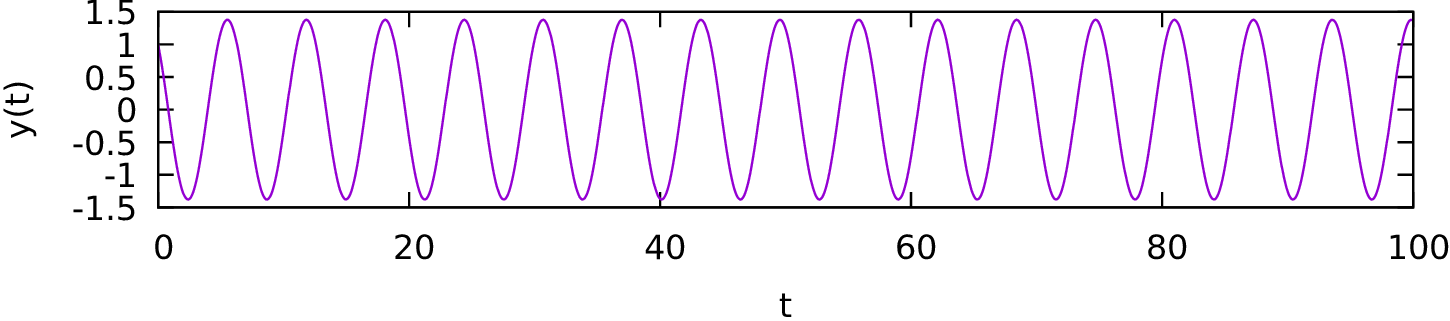
Fig. 3.1 Output for the simple harmonic oscillator problem