3.6.5. Temporal adaptivity
It is not always easy to find a good time step that is sufficiently accurate. Of course, you can make a guess and rerun the simulation with reduced time step to see whether the dynamics is affected by the time step. If not, you might have found a good time step. However, some systems have unpredictable dynamics, as e.g. chaotic systems, which might show very strongly fluctuating dynamics.
pyoomph allows to flexibly adjust the time step during the simulation depending on an estimate of the error the current time step might have. To that end, the next time step is first predicted based on the previous steps, then a step is taken and the result is compared with the prediction. If the difference is too large, pyoomph will discard this step and retries with a smaller time step. At the same time, if the prediction and the computed solution match very well, pyoomph gradually tries to increase the time step.
Here, we will use the chaotic Lorenz system, known for its chaotic strange attractor, to illustrate this feature. The Lorenz system consists of three coupled non-linear ODEs of first order
with three parameters \((\sigma,\rho,\beta)\). Implementing this in pyoomph is trivial:
class LorenzSystem(ODEEquations):
     def __init__(self,*,sigma=10,rho=28,beta=8/3,scheme="BDF2"): # Default parameters used by Lorenz
             super(LorenzSystem,self).__init__()
             self.sigma=sigma
             self.rho=rho
             self.beta=beta
             self.scheme=scheme

     def define_fields(self):
             self.define_ode_variable("x","y","z")

     def define_residuals(self):
             x,y,z=var(["x","y","z"])
             residual=(partial_t(x)-self.sigma*(y-x))*testfunction(x)
             residual+=(partial_t(y)-x*(self.rho-z)+y)*testfunction(y)
             residual+=(partial_t(z)-x*y+self.beta*z)*testfunction(z)
             self.add_residual(time_scheme(self.scheme,residual))


class LorenzProblem(Problem):
To add the feature of temporal adaptivity to the system, it is sufficient to combine the equations with a TemporalErrorEstimator
class LorenzProblem(Problem):

     def define_problem(self):
             eqs=LorenzSystem(scheme="BDF2") # Temporal adaptivity works best with BDF2
             eqs+=InitialCondition(x=0.01)  # Some non-trivial initial position
             eqs+=TemporalErrorEstimator(x=1,y=1,z=1) # Weight all temporal error with unity
             eqs+=ODEFileOutput()
             self.add_equations(eqs@"lorenz_attractor")
TemporalErrorEstimator takes keyword arguments of the form variable_name=error_weight, i.e. we can set to each of the ODE variables a different weighting for the computation of the temporal error between prediction and actual solution. In the code here, all weights have been set to unity, i.e. all variables \(x\), \(y\), \(z\) are weighted equally in the determination of the temporal error.
Finally, the run() statement takes a keyword argument temporal_error, which defined the error we are ready to accept. The smaller the temporal error, the finer the dynamics time steps, but the longer the computation takes.
if __name__=="__main__":
     with LorenzProblem() as problem:
             # outstep=True means output every step
             # startstep is the first time step
             # temporal_error controls the maximum difference between prediction and actual result
             problem.run(endtime=100,outstep=True,startstep=0.0001,temporal_error=0.005)
Note the also outstep=True was passed instead of numouts. It will just output each step. Of course, also a startstep should be set so that the problem has a good guess how to start. If the value of temporal_error is set too large, the system might not show the correct dynamics, see Fig. 3.6. The accepted time steps are displayed in Fig. 3.7.
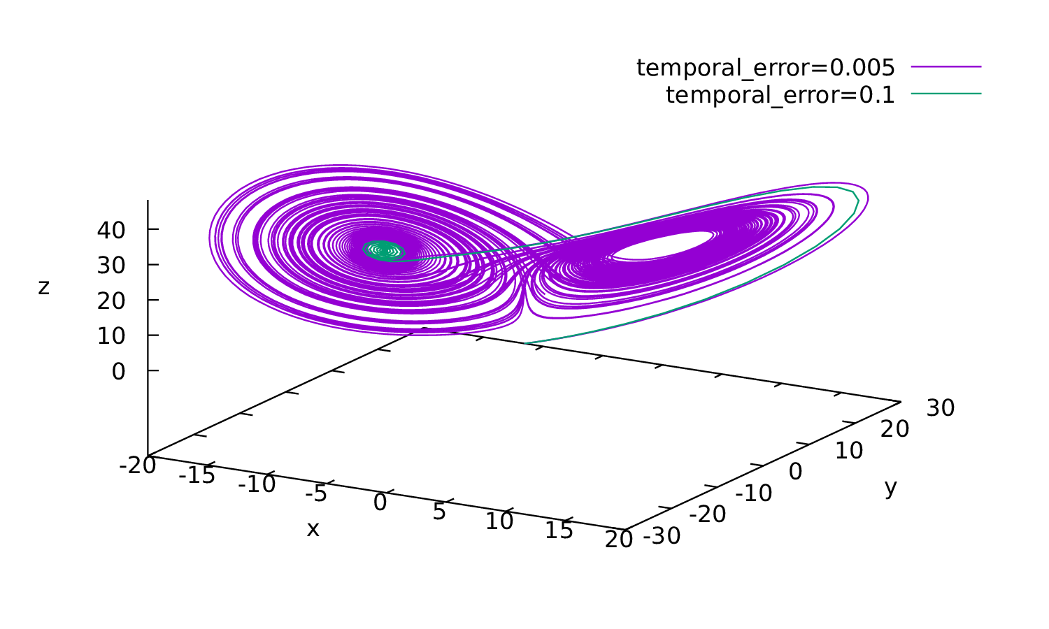
Fig. 3.6 Dynamics of the Lorenz system with adaptive time stepping. Allowing too large errors will give the wrong dynamics.

Fig. 3.7 Accepted time steps in the case of temporal_error=0.005