3.11.1. Global parameters
Let us discuss the procedure on the basis of the transcritical normal form, which reads
where \(r\) is the parameter. As usual, the stationary solutions can be obtained by setting \(\partial_tx=0\), which yields the two stationary solutions \(x_{0}=0\) and \(x_{0}=r\). The stability of these solutions can also be assessed easily by hand. One just introduces a perturbed solution \(x(t)=x_0+\delta x(t)\) and linearizes the dynamics of \(\delta x\):
Obviously, when \(r\) passes \(0\), the dynamics of the system changes. For \(r<0\), the stationary solution \(x_0=0\) is stable and \(x_0=r\) is unstable, whereas it is vice versa for \(r>0\).
In pyoomph, we again formulate the very simple equation class for this, passing some value (or expression) as parameter r:
class TranscriticalNormalForm(ODEEquations):
    def __init__(self,r):
        super(TranscriticalNormalForm, self).__init__()
        self.r=r

    def define_fields(self):
        self.define_ode_variable("x")

    def define_residuals(self):
        x,x_test=var_and_test("x") #Shortcut to get var("x") and testfunction("x")
        self.add_residual((partial_t(x)-self.r*x+x**2)*x_test)
In the problem class, we use define_global_parameter() to define a global parameter object with an initial value. This parameter is defined on the problem level. When combined in an expression, automatically its symbolical (i.e. adjustable) value will be used. However, unlike var(), parameters are not considered to be unknowns of the system. To adjust the value of a parameter, we can access the current value by the property value. If we apply float() to an expression containing a parameter, the current value will be substituted.
class TranscriticalProblem(Problem):
    def __init__(self):
        super(TranscriticalProblem, self).__init__()
        # Bifuraction parameter with default value
        self.r=self.define_global_parameter(r=1)
        self.x0=1

    def define_problem(self):
        eq=TranscriticalNormalForm(r=self.r) #Pass the symbolic 'r' here
        eq+=InitialCondition(x=self.x0)
        eq+=ODEFileOutput()
        self.add_equations(eq@"transcritical")
Let us first run the problem as before, namely by using the run() method of the Problem class:
if __name__=="__main__":
    with TranscriticalProblem() as problem:

        problem.r.value=1 # You can set the value here
        problem.x0=0.001 # Start slightly above the unstable solution x=0
        problem.run(endtime=20,numouts=100) # And let it evolve towards the stable branch x=r

        problem.r.value=-1 # Change the parameter value, x=1 is now not a stationary solution anymore
        problem.run(endtime=40, numouts=100)  # And let it evolve towards the now stable branch x=0
We first set \(r=1\), but start close to the unstable branch \(x=0\). In the output, we will see an initial exponential growth of \(x(t)\), followed by a convergence into the stable branch at \(x=r=1\). However, after \(t=20\), we change the parameter value. This feature, i.e. modifying a system parameter, is only possible with parameters as constructed here. Changes in other properties, e.g. the initial condition \(x_0\) or the harmonic oscillator frequency \(\omega\) in the first examples within this book have no effect after the problem has been initialized, since the code is generated based on the values at the beginning. However, global parameters are still variables within the generated code and they are re-evaluated every single time step. Therefore, it is possible to change the value of \(r\) in between.
After setting \(r=-1\), the dynamics of the system entirely changes. In particular, the branch \(x_0=1\), which the solution was just trying to attain, has now moved to \(x_0=-1=r\). Furthermore, as discussed before, \(x=0\) has now become the stable branch. Therefore, the output for \(t>20\), generated by the second run() statement, will show how \(x\) approaches \(0\) instead, see Fig. 3.12.
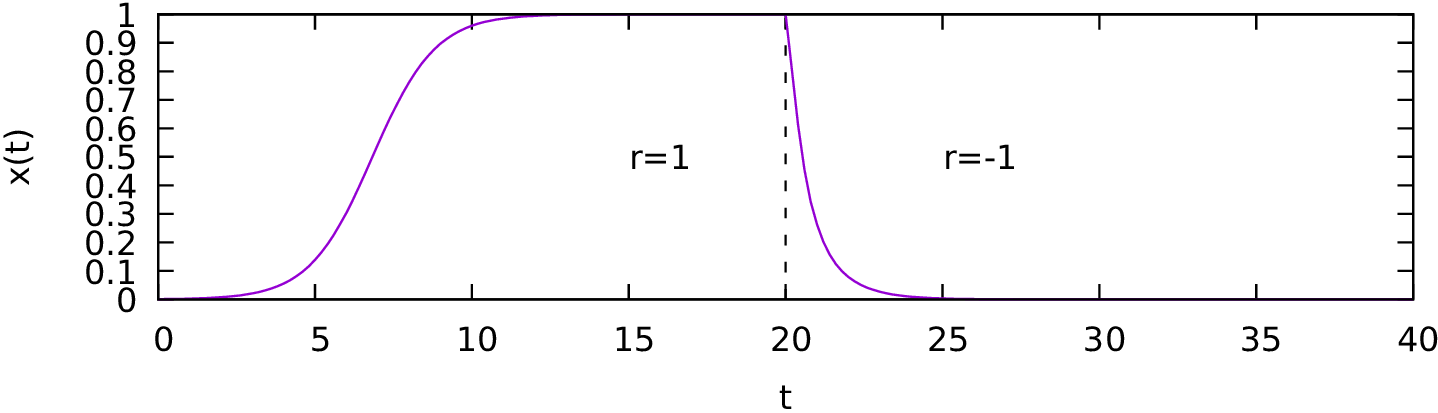
Fig. 3.12 Temporal integration of the transcritical normal form with a switch of the parameter \(r\) at \(t=20\). Depending on \(r\), the stationary solution at \(x=0\) is either unstable or stable.