7.4. Connecting two fluid domains
In Section 6.5, we have developed the equations of a free liquid surface. However, so far we have not considered the presence of the opposite side of the free surface, which is usually also a fluid. So let’s do this now…
Let us consider two phases "inside" and "outside" with respect to the free surface, which we will address by "interface" or "inside/interface", since we will add all necessary InterfaceEquations on the "interface" from the domain "inside". Actually, the kinematic boundary condition (6.4) has to be fulfilled on both sides. When we use again a phase superscript \(\phi\), we can state
where the normal \(\vec{n}^\text{i}\) is pointing from "inside" to "outside" (actually, which direction does not matter here). However, if one just adds one KinematicBC object per side, i.e. on "inside/interface" and "outside/interface", the kinematic boundary condition would be fulfilled on both sides, but once the mesh is connected with a ConnectMeshAtInterface object, the normal mesh motion would be over-constrained.
Both kinematic boundary conditions together can be also formulated by the kinematic boundary condition for the "inside" domain and the requirement that the normal velocity is continuous across the "interface":
When we further demand that the tangential velocity should be also continuous (which is a reasonable assumption), (7.7) reads
which can be enforced by a vectorial Lagrange multiplier field \(\vec\lambda\) (with test function \(\vec{\eta}\)) as usual
The dynamic boundary condition (6.6) must be generalized to
where the lhs can be simplified due to \(\vec{n}^\text{i}=-\vec{n}^\text{o}\). Indeed, analogous to the heat flux in Section 7.1, this equation is automatically fulfilled if we add a DynamicBC to the "inside/interface" and couple the velocities on both sides via (7.9): On the "inside/interface", we then have the Neumann contribution
and on the "outside/interface"
It is apparent that the sum of the latter two equations indeed gives the dynamic boundary condition (7.10).
So the only additional work we have to do is to couple the velocities by a Lagrange multiplier, which can be implemented in pyoomph as
from pyoomph import *
from pyoomph.expressions import *
from pyoomph.equations.navier_stokes import *
from pyoomph.equations.ALE import *

class EnforceContinuousVelocity(InterfaceEquations):
	def define_fields(self):
		self.define_vector_field("_couple_velo","C2")

	def define_residuals(self):
		l,ltest=var_and_test("_couple_velo")
		ui,uitest=var_and_test("velocity") # inner velocity at the interface
		uo,uotest=var_and_test("velocity",domain=self.get_opposite_side_of_interface()) # outer velocity
		self.add_residual(weak(ui-uo,ltest)+weak(l,uitest)-weak(l,uotest))

	def before_assigning_equations_postorder(self, mesh):
		# pin Lagrange multiplier if both velocities are pinned
		# we have to iterate over the directions x,y,z (if present)
		for d in ["x","y","z"][0:self.get_nodal_dimension()]:
			self.pin_redundant_lagrange_multipliers(mesh,"_couple_velo_"+d,"velocity_"+d,opposite_interface="velocity_"+d)
Again, we have to tell var() with domain=self.get_opposite_side_of_interface() that we want to have the outer velocity field, whereas without this argument, the inner velocity is meant. When both velocities are prescribed with a DirichletBC, i.e. pinned, the Lagrange multiplier would either lead to a null space (if the strongly imposed velocities are matching) or to the absence of any solution (if the strongly imposed velocities are mismatching). We have to do this per component, which is done in the for loop. Here, only the components are considered, which are actually present in the actual nodal dimension of the mesh via get_nodal_dimension(). We also use the argument opposite_interface=... to tell pin_redundant_lagrange_multipliers() that each component of the Lagrange multiplier \(\vec\lambda\) is only redundant if both the inside and the outside velocity components are pinned. Note that the predefined InterfaceEquations class ConnectMeshAtInterface does exactly the same but on the mesh positions.
The rest of the code is rather straight-forward; however, we use the RectangularQuadMesh with a lambda callable as argument for name:
class TwoLayerFlowProblem(Problem):
	def __init__(self):
		super(TwoLayerFlowProblem, self).__init__()
		self.W=1
		self.H1=0.1
		self.H2=0.1
		self.quad_size=0.01

	def define_problem(self):
		domain_names=lambda x,y: "lower" if y<self.H1 else "upper" # Name lower half lower, upper half upper
		self.add_mesh(RectangularQuadMesh(N=[math.ceil(self.W/self.quad_size), math.ceil((self.H1+self.H2)/self.quad_size)], size=[self.W, self.H1+self.H2],name=domain_names,boundary_names={"lower_upper":"interface"}))
With this argument, we can split the RectangularQuadMesh into multiple domains. The callable passed to name receives nondimensional \(x,y\) coordinates of the element centers and is expected to return the name of the domain. Interfaces between the different domains are automatically marked by "domain1_domain2" with the adjacent domain names "domain1" and "domain2" (in alphabetical order). Here, we rename this interface "lower_upper" via the boundary_names dict to "interface".
The equations are assembled and added:
		# Add the same required equations to both domains
		for dom in ["lower","upper"]:
			eqs=LaplaceSmoothedMesh()
			eqs+=MeshFileOutput()
			eqs+=DirichletBC(mesh_x=True)
			eqs += DirichletBC(velocity_x=0) @ "left"  # no in/outflow at the sides
			eqs += DirichletBC(velocity_x=0) @ "right"
			self.add_equations(eqs@dom)

		# Different fluids
		l_eqs = NavierStokesEquations(mass_density=0.01, dynamic_viscosity=1)  # NS equations
		u_eqs = NavierStokesEquations(mass_density=0.01, dynamic_viscosity=0.01)  # NS equations

		# no slip at top and bottom
		l_eqs += DirichletBC(velocity_x=0, velocity_y=0, mesh_y=0) @ "bottom"  # no slip at bottom and fix the mesh there
		u_eqs += DirichletBC(velocity_x=0, velocity_y=0, mesh_y=self.H1+self.H2) @ "top"  # no slip at bottom and fix the mesh there
		l_eqs += DirichletBC(pressure=0) @"bottom/left" # pin one pressure degree

		# Free surface, mesh connection and velocity connection
		l_eqs += NavierStokesFreeSurface(surface_tension=1) @ "interface"  # free surface at the top
		l_eqs += ConnectMeshAtInterface()@"interface"
		l_eqs += EnforceContinuousVelocity()@"interface"

		# Deform the initial mesh
		X, Y = var(["lagrangian_x", "lagrangian_y"])
		l_eqs += InitialCondition(mesh_y=Y * (1 + 0.25 * cos(2 * pi * X)))  # small height with a modulation
		u_eqs += InitialCondition(mesh_y=Y+ (self.H1+self.H2-Y)*(0.25 * cos(2 * pi * X)))  # small height with a modulation
		self.add_equations(l_eqs @ "lower" + u_eqs @ "upper")  # adding it to the system
We use the predefined NavierStokesFreeSurface instead of our free surface consisting of KinematicBC and DynamicBC developed in Section 6.5, but it does essentially the same. With the EnforceContinuousVelocity, the velocities are enforced to be continuous, whereas the Lagrange multiplier \(\lambda_x\) in \(x\)-direction will be pinned to \(0\) automatically on the "left" and "right", since both inside and outside velocities are prescribed by a DirichletBC.
The run code reads
if __name__=="__main__":
	with TwoLayerFlowProblem() as problem:
		problem.run(50,outstep=True,startstep=0.25)
and the results are depicted in Fig. 7.4.
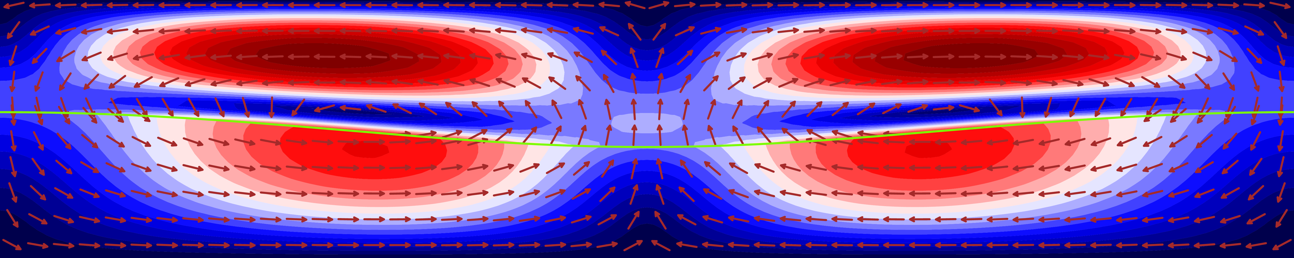
Fig. 7.4 Two-layer flow with connected velocity at the interface. By the velocity coupling, the stress is correctly distributed between both domains.
Tip
There is a similar example case in oomph-lib at https://oomph-lib.github.io/oomph-lib/doc/navier_stokes/two_layer_interface/html/index.html. However, in their case, a single mesh (i.e. domain) is used, but with varying viscosity and mass densities per element. The free surface is just added at an interior interface. Thereby, the continuity of the velocity field and the mesh position across the interface is automatically fulfilled, i.e. no Lagrange multipliers to connect the velocity and mesh are necessary. However, since the pressure has a jump at the interface due to the Laplace pressure, the pressure space must be discontinuous, i.e. in the oomph-lib example, Crouzeix-Raviart instead of Taylor-Hood elements are used. While it is possible to follow the same approach in pyoomph, it is not discussed here. The moment mass transfer between both phases is considered, the normal velocity has a jump at the interface as well, provided the mass densities in both phases are different. Then, Lagrange multipliers are definitely required.
If you are interested in a pyoomph version of oomph-lib’s way of implementing it on a single domain, you find the corresponding code here: two_layer_flow_single_domain.py