7.2. Propagation of an ice front
The next problem is very related to the previous one. We will again solve two temperature conduction equations, but this time, condition (7.2) will be slightly different. Furthermore, we will consider also the temporal behavior and use physical dimensions.
In fact, we want to solve the propagation of an ice front, i.e. how ice is solidifying or melting in the presence of a temperature gradient. Since this phase transition obviously leads to a growth of the ice domain and a corresponding shrinkage of the liquid domain or vice versa, a moving mesh/ALE method will be used.
Mathematically, we have the transient heat conduction equations
where the phase superscript \(\phi\) can be either ice or liquid, depending on whether we apply this equation on either the "ice" or the "liquid" domain. The equation can be easily cast into its weak form and implemented:
from temperature_conduction import *	# To get the mesh from the previous example
from pyoomph.expressions.units import * # units for dimensions
from pyoomph.equations.ALE import * # moving mesh equations


class ThermalConductionEquation(Equations):
    def __init__(self,k,rho,c_p):
        super(ThermalConductionEquation,self).__init__()
        # store conductivity, mass density and spec. heat capacity
        self.k,self.rho,self.c_p=k,rho,c_p

    def define_fields(self):
        # Note the testscale here: We want to nondimensionalize the entire equation by the scale "thermal_equation"
        # which will be set at the problem level
        self.define_scalar_field("T","C2",testscale=1/scale_factor("thermal_equation"))

    def define_residuals(self):
        T,T_test=var_and_test("T")
        self.add_residual(weak(self.rho*self.c_p*partial_t(T),T_test)+weak(self.k*grad(T),grad(T_test)))
Note that we bind the test scale of the temperature field "T" to 1/scale_factor("thermal_equation"). This means essentially, that (7.3) is multiplied by a factor \(1/S\) during non-dimensionalization, i.e. that we actually solve
One could now choose e.g. \(S=\rho^\text{ice} c_p^\text{ice} [T]/[t]\), where \([T]\) is the scaling of the temperature field, e.g. \(1\:\mathrm{K}\) and \([t]\) is the characteristic time scale, e.g. \(1\:\mathrm{s}\). Thereby, the nondimensional lhs would have a unity factor. Alternatively, we can also set the factor of the nondimensional conduction term on the rhs to unity by selecting \(S=k^\text{ice}[T]/[X]^2\) with the spatial scale \(X\). Of course, one can also use the properties of the "liquid" domain instead of the "ice" domain. Eventually, \(S\) will be set at Problem level with the set_scaling(thermal_equation=...) method. Thereby, on both domains, the equations will have the same test scale, i.e. are nondimensionalized with respect to the same scale. That way, the problem regarding the consistency of the heat flux at the interface, as discussed in the previous example, will be circumvented. Therefore, this approach is a good practice.
Next, we must couple the interface motion, i.e. the propagation of the ice front, with the heat fluxes. The interface \(x_\text{I}\) will move, according to
where \(\Lambda\) is the latent heat of solidification. We have used \(\rho^\text{ice}\) in the denominator, since the liquid will actually be subject to a tiny normal velocity at the interface due to the density difference. But this small contribution is disregarded here, since only conduction equations are solved.
As usual in pyoomph, we should write this equation independent of the chosen coordinate system to make this equation applicable to any problem. This is obviously given by
In this formulation with interface normal \(\vec{n}\), we also notice that it is a constraint for the normal motion of the mesh, whereas the tangential motion is not affected. Since it is a constraint, the typical Lagrange multiplier approach is again the way to take. As usual, with \(\vec{\chi}\) and \(\eta\) being the test functions of the mesh position and the Lagrange multiplier \(\lambda\), respectively, we get the weak formulation for the constraint:
The implementation is rather straight-forward:
class IceFrontSpeed(InterfaceEquations):
    required_parent_type=ThermalConductionEquation	# Must have ThermalConductionEquation on the inside bulk
    required_opposite_parent_type = ThermalConductionEquation # and ThermalConductionEquation on the outside bulk

    def __init__(self,latent_heat):
        super(IceFrontSpeed, self).__init__()
        self.latent_heat=latent_heat

    def define_fields(self):
        self.define_scalar_field("_lagr_interf_speed","C2",scale=1/test_scale_factor("mesh"),testscale=scale_factor("temporal")/scale_factor("spatial"))

    def define_residuals(self):
        n=var("normal")
        x,xtest=var_and_test("mesh")
        l,ltest=var_and_test("_lagr_interf_speed")
        k_in=self.get_parent_equations().k		# conductivity of the inside domain
        rho_in=self.get_parent_equations().rho	# density of the inside domain
        k_out=self.get_opposite_parent_equations().k # conductivity of the outside domain
        T_bulk_in=var("T",domain=self.get_parent_domain())	# temperature in the inside bulk
        T_bulk_out = var("T", domain=self.get_opposite_parent_domain()) # temperature in the outside bulk
        speed=dot(k_in*grad(T_bulk_in)-k_out*grad(T_bulk_out),n)/(rho_in*self.latent_heat)
        self.add_residual(weak(dot(mesh_velocity(),n)-speed,ltest))
        self.add_residual(weak(l,dot(xtest,n)))
With the required_parent_type and required_opposite_parent_type, we inform pyoomph that it is only allowed to attach this constraint to an interface that has a TemperatureConductionEquation on both the inside bulk and the outside bulk of this interface. Otherwise, an error will be thrown. Due to these statements, we also get automatically the inside and outside TemperatureConductionEquation of the bulk phases when calling get_parent_equations() and get_opposite_parent_equations(). This is used to obtain the required properties \(k^\phi\) and \(\rho\) in the define_residuals() method here. The interface property latent_heat, however, has to be passed to the constructor and is stored internally.
The scaling has to fit, i.e. upon non-dimensionalization of (7.5), all weak forms must yield non-dimensional results. Indeed, if we scale \(\lambda\) with the inverse of the scaling of \(\chi\) and nondimensionalize the test function \(\eta\) as \(\eta=[T]/[X]\tilde\eta\), all units will cancel out in (7.5).
There is another very relevant aspect to consider, namely:
Warning
One fundamental aspect is that we want to take the bulk gradient for the \(\nabla T\) terms in (7.5). Since we are on an interface, i.e. on a manifold with co-dimension 1, the simple statement grad(var("T")) would expand to the surface gradient \(\nabla_S T\) of the temperature field of the inside domain (cf. Section 4.3.2), which will be always tangential to \(\vec{n}\). The bulk gradients are only obtained if the temperature fields of the bulk phases are passed to grad(). These can be obtained by adding get_parent_domain() and get_opposite_parent_domain() (for the inside and outside bulk, respectively) as domain= keyword argument in the bindings via var().
Alternatively, you can also use domain=".." instead of domain=self.get_parent_domain() and domain="|.." instead of domain=self.get_opposite_parent_domain().
In the constructor of the Problem class, nothing spectacular happens. We just initialize a few default parameters:
class IceFrontProblem(Problem):
    def __init__(self):
        super(IceFrontProblem,self).__init__()

        # properties of the ice
        self.rho_ice=915*kilogram/(meter**3) # mass density
        self.k_ice=2.22*watt/(meter*kelvin) # thermal conductivity
        self.cp_ice=2.050*kilo*joule/(kilogram*kelvin)	# spec. heat capacity

        # properties of the liquid
        self.rho_liq=999.87*kilogram/(meter**3)
        self.k_liq=0.5610*watt/(meter*kelvin)
        self.cp_liq=4.22*kilo*joule/(kilogram*kelvin)

        self.T_eq=0*celsius # Melting point
        self.latent_heat= 334 *joule/gram # Latent heat of melting/solidification

        self.L=1*milli*meter # domain length
        self.front_start_fraction=0.3 # initial relative position of the front
        self.T_left=-1*celsius # left and right temperatures
        self.T_right=1*celsius
In the define_problem() method, we have to set the scales for nondimensionalization and we make use of a for loop to construct similar equations on both domains:
    def define_problem(self):
        # Mesh: a dimensional size and xI is set, also the domains are renamed
        self.add_mesh(TwoDomainMesh1d(L=self.L,xI=self.L*self.front_start_fraction,left_domain_name="ice",right_domain_name="liquid"))
        self.set_scaling(spatial=self.L,temporal=100*second) # Nondimensionalize space and time by these quantities
        self.set_scaling(T=kelvin) # Temperature scale
        # Now, we define the scale "thermal_equation", by what both thermal equations will be divided
        # We take the conduction term of the ice as reference here
        self.set_scaling(thermal_equation=scale_factor("T")*self.k_ice/scale_factor("spatial")**2)

        # Create similar equations on both domains
        # wrap the domain name and the corresponding properties
        domain_props=[["ice",self.k_ice,self.rho_ice,self.cp_ice,self.T_left],
                      ["liquid",self.k_liq,self.rho_liq,self.cp_liq,self.T_right]]
        for (domain_name,k,rho,cp,T_init) in domain_props: # iterate over the entries
            eqs=TextFileOutput() # Output
            eqs+=ThermalConductionEquation(k,rho,cp) # thermal transport eq
            eqs+=LaplaceSmoothedMesh()  # mesh motion
            eqs+=InitialCondition(T=T_init) # initial condition
            eqs+=SpatialErrorEstimator(T=1) # spatial adaptivity
            eqs+=DirichletBC(T=self.T_eq)@"interface" # melting point at the interface
            self.add_equations(eqs@domain_name) # add the equations

        # Dirichlet conditions
        self.add_equations(DirichletBC(T=self.T_left,mesh_x=0)@"ice/left")
        self.add_equations(DirichletBC(T=self.T_right,mesh_x=self.L)@"liquid/right")

        # Interface equations
        interf_eqs=IceFrontSpeed(self.latent_heat) # Front speed equation
        interf_eqs+=ConnectMeshAtInterface() # Connect the mesh at xI

        # We could also add it on "liquid/interface", but then we must use -self.latent_heat in the IceFrontSpeed
        self.add_equations(interf_eqs@"ice/interface")
The interface equations consist of an instance of our just developed class IceFrontSpeed and the predefined class ConnectMeshAtInterface. The latter will introduce Lagrange multipliers so that the nodes of the "liquid" and "ice" domain at the mutual "interface" will be enforced to coincide. Without this, only the "ice" mesh would move, whereas the "liquid" mesh would remain static. As an alternative to adding interf_eqs@"ice/interface" to the problem, we could also add interf_eqs to the "liquid" side of the "interface". In that case, however, we would have to negate the latent_heat.
The code to run this problem is simple, but we use temporal and spatial adaptivity to properly resolve the initial temperature discontinuity at the "interface":
if __name__=="__main__":
    with IceFrontProblem() as problem:
        problem.run(1000*second,startstep=0.00001*second,outstep=True,temporal_error=1,spatial_adapt=1,maxstep=2*second)
The results are shown in Fig. 7.2.
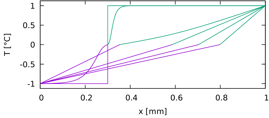
Fig. 7.2 Propagation of the front between solid ice (left) and liquid water (right) due to a temperature gradient at different times.