6.5. Free surface Navier-Stokes equation
We will now combine the Laplace smoothed moving mesh with a Navier-Stokes equation. Having a moving mesh allows us to track a free surface and impose a surface tension on it. We will have two boundary conditions that must be enforced, namely the kinematic and the dynamic boundary condition.
The kinematic boundary condition reads
i.e. the mesh has to move with the normal fluid velocity [5]. This is obviously a constraint which narrows the potential solutions of the mesh coordinates. We therefore add a field of Lagrange multipliers \(\lambda\) with test function \(\eta\) on each free surface that enforces this constraint. Since we want the normal mesh motion to follow the fluid, and not the velocity following the mesh motion, we add the action of the Lagrange multiplier to the test space of the mesh, not the velocity. If we would add it to the test space of the velocity, the particular mesh equations (e.g. the Laplace smoothed mesh) would influence the flow, which is not reasonable. Hence, the weak form at the free surfaces for the kinematic boundary condition reads
The implementation of the kinematic boundary condition could read as follows
from pyoomph import *

# use the pre-defined Navier-Stokes ( it will use partial_t(...,ALE="auto") )
from pyoomph.equations.navier_stokes import *
# and the pre-defined LaplaceSmoothedMesh
from pyoomph.equations.ALE import *

class KinematicBC(InterfaceEquations):
     def define_fields(self):
             self.define_scalar_field("_kin_bc","C2") # second order field lambda

     def define_residuals(self):
             n,u=var(["normal","velocity"])
             l,eta=var_and_test("_kin_bc") # Lagrange multiplier
             x,chi=var_and_test("mesh") # unknown mesh coordinates
             # Let the normal mesh velocity follow the normal fluid velocity
             self.add_residual(weak(dot(n,u-mesh_velocity()),eta)-weak(l,dot(n,chi)))

     def before_assigning_equations_postorder(self, mesh):
             # pin the Lagrange multiplier, when the mesh is locally entirely pinned
             self.pin_redundant_lagrange_multipliers(mesh, "_kin_bc", "mesh")
Note that we use mesh_velocity() instead of partial_t() to calculate the mesh velocity. In fact, mesh_velocity() is just partial_t(var("mesh"),ALE=False). This is reasonable, since we want the mesh velocity co-moving with the interface, i.e. directly at the nodes.
Again, we use pin_redundant_lagrange_multipliers() in the before_assigning_equations_postorder() method to automatically pin the local Lagrange multiplier, if the mesh position is entirely pinned at any node. If the mesh cannot move, the Lagrange multiplier would otherwise over-constrain the problem.
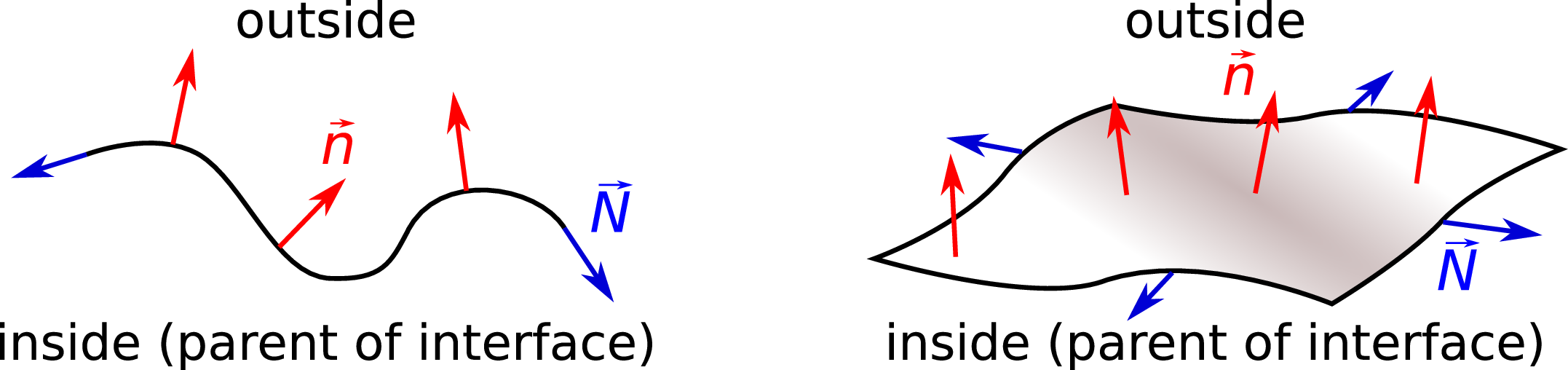
Fig. 6.4 Interface normals \(\vec{n}\) (normal to the interface, pointing outside from the parent domain) and the interface boundary normals \(\vec{N}\) (tangentially to the interface, pointing outwards) for a 1d interface of a 2d bulk domain and a 2d interface of a 3d bulk domain.
The second condition is the dynamic boundary condition. This one states that the traction is given by a combination of the interface curvature \(\kappa\), the surface tension \(\sigma\) and potential tangential gradients of the latter, i.e.
\(\nabla_S\) is the surface gradient operator, sometimes written as \(\nabla_S=\left(\mathbf{1}-\mathbf{nn}\right)\nabla\), and will only have tangential contributions. Obviously, the lhs of this equation is the negative Neumann contribution we can add to the (Navier-)Stokes equation, cf. (4.13). It could be hence implemented by adding
as interface contribution to the velocity test function \(\vec{v}\). However, it is not trivial to calculate the curvature \(\kappa=-\nabla_S\cdot \vec{n}\). In fact, pyoomph does not allow to calculate the surface divergence of the normal yet. Instead, we make use of the surface divergence theorem. For an arbitrary vector field \(\vec{w}\) defined on the interface \(\Gamma\), we have the relation
where the last integral is comprising the boundary of the surface with outward normal \(\vec{N}\) (cf. Fig. 6.4 for an illustration of both kinds of normals). When selecting \(\vec{w}=\sigma\vec{v}\), this can be arranged to
or, alternatively, using the product rule
and by moving the surface tension gradient \(\nabla_S \sigma\) from the right to the left, we get
Upon negation, we can identify the weak forms
So instead calculating the curvature, it is sufficient to add \(\langle \sigma, \nabla_S\cdot\vec{v}\rangle\) to get both normal traction due to the Laplace pressure and tangential Marangoni stresses simultaneously. Additionally, there is another term \([\cdot,\cdot]\) arising, which allows weak Neumann contributions at the ends of the free surface, which will help us to impose contact angles soon.
Tip
oomph-lib also covers the boundary conditions of a free surface in the tutorial at https://oomph-lib.github.io/oomph-lib/doc/navier_stokes/surface_theory/html/index.html.
Also, an analogous implementation of the following free surface can be found in oomph-lib at https://oomph-lib.github.io/oomph-lib/doc/navier_stokes/single_layer_free_surface/html/index.html
But first, let us now implement the dynamic boundary condition which can be added to the free surface itself, i.e. the \(\langle \cdot , \cdot \rangle\) contribution:
class DynamicBC(InterfaceEquations):
     def __init__(self,sigma):
             super(DynamicBC,self).__init__()
             self.sigma=sigma

     def define_residuals(self):
             v=testfunction("velocity")
             self.add_residual(weak(self.sigma,div(v)))
One might wonder whether div() is indeed the surface divergence operator \(\nabla_S\). But when this equation is added to an interface, it will indeed expand to this. There is no other reasonable way to calculate the divergence of a field defined on a manifold embedded in a higher order space. The same applies for grad(): In the bulk, i.e. on domains with zero co-dimension, it is indeed the convectional gradient, but on manifolds (surfaces) with nonzero co-dimension, it will be the corresponding surface gradient.
Before defining the problem, we can combine both boundary conditions in a short-hand notation:
# Shortcut to create both conditions simultaneously
def FreeSurface(sigma):
     return KinematicBC()+DynamicBC(sigma)
Now, as example problem, let us do the same as before on the basis of lubrication theory in Section 5.4.1, but this time solving the exact flow and the exact free surface dynamics:

Fig. 6.5 Free surface combined with Navier-Stokes and a Laplace-smoothed mesh.
class SurfaceRelaxationProblem(Problem):
     def define_problem(self):
             # Shallow 2d mesh
             self.add_mesh(RectangularQuadMesh(N=[80,4],size=[1,0.05]))
             eqs=NavierStokesEquations(mass_density=0.01,dynamic_viscosity=1) # equations
             eqs+=LaplaceSmoothedMesh() # Laplace smoothed mesh
             eqs+=DirichletBC(mesh_x=True) # We can fix all x-coordinates, since the problem is rather shallow
             eqs+=MeshFileOutput() # output
             eqs+=DirichletBC(velocity_x=0,velocity_y=0,mesh_y=0)@"bottom" # no slip at bottom and fix the mesh there
             eqs+=DirichletBC(velocity_x=0)@"left" # no in/outflow at the sides
             eqs+=DirichletBC(velocity_x=0)@"right"
             eqs+=FreeSurface(sigma=1)@"top" # free surface at the top
             # Deform the initial mesh
             X,Y=var(["lagrangian_x","lagrangian_y"])
             eqs+=InitialCondition(mesh_y=Y*(1+0.25*cos(2*pi*X)))  # small height with a modulation
             self.add_equations(eqs@"domain") # adding it to the system


if __name__=="__main__":
     with SurfaceRelaxationProblem() as problem:
             problem.run(50,outstep=True,startstep=0.25)
Opposed to the lubrication example in Section 5.4.1, we use a RectangularQuadMesh to resolve the entire bulk flow. We add the predefined NavierStokesEquations, which also - opposed to lubrication theory - allows for inertia due to the finite mass density. In order to use the free surface equations we have just defined, we must allow the mesh nodes to move, since the KinematicBC requires to add weak contributions to the test function of the mesh coordinates. We therefore use the predefined LaplaceSmoothedMesh. However, since this particular problem is shallow, it is sufficient to only consider motion in \(y\)-direction. This can be achieved by just pinning all \(x\)-positions to their initial values by the DirichletBC(mesh_x=True). We impose no slip and a zero \(y\)-coordinate at the "bottom" interface and prevent any in- or outflow at the "left" and "right" interfaces. Finally, we deform the initial mesh by adding an InitialCondition, which sets the \(y\)-position based on the "lagrangian" coordinate, which corresponds to the undeformed mesh by default.