7.6. Evaporation of a sessile droplet
Evaporation, as mass transfer between phases in general, always requires more than a single phase. We have seen how we can couple different equations on individual domains and hence we can solve evaporating sessile droplets. To that end, we have to solve the Navier-Stokes equation for the droplet, the interface dynamics and for the gas phase, the diffusion equation of the vapor field. While there is actually also advective vapor transport, it usually negligible for temperatures below the boiling point.
First of all, we must have a mesh that comprises a sessile droplet and a surrounding gas domain:
from pyoomph import *
from pyoomph.equations.ALE import * # Moving mesh
from pyoomph.equations.navier_stokes import * # Flow
from pyoomph.expressions.units import * # units
from pyoomph.utils.dropgeom import  * # utils to calculate droplet contact angle from height and radius, etc.
from pyoomph.equations.advection_diffusion import * # for the gas diffusion
from pyoomph.meshes.remesher import * # to remesh at large distortions


# A mesh of an axisymmetric droplet surrounded by gas
class DropletWithGasMesh(GmshTemplate):
    def __init__(self,droplet_radius,droplet_height,gas_radius,cl_resolution_factor=0.1,gas_resolution_factor=50):
        super(DropletWithGasMesh, self).__init__()
        self.droplet_radius,self.droplet_height,self.gas_radius=droplet_radius,droplet_height,gas_radius
        self.cl_resolution_factor,self.gas_resolution_factor=cl_resolution_factor,gas_resolution_factor
        self.default_resolution=0.025
        #self.mesh_mode="tris"

    def define_geometry(self):
        # finer resolution at the contact line, lower at the gas far field
        res_cl=self.cl_resolution_factor*self.default_resolution
        res_gas=self.gas_resolution_factor*self.default_resolution
        # droplet
        p00=self.point(0,0) # origin
        pr0 = self.point(self.droplet_radius, 0,size=res_cl) # contact line
        p0h=self.point(0,self.droplet_height) # zenith
        self.circle_arc(pr0,p0h,through_point=self.point(-self.droplet_radius,0),name="droplet_gas") # curved interface
        self.create_lines(p0h,"droplet_axisymm",p00,"droplet_substrate",pr0)
        self.plane_surface("droplet_gas","droplet_axisymm","droplet_substrate",name="droplet") # droplet domain
        # gas dome
        pR0=self.point(self.gas_radius,0,size=res_gas)
        p0R = self.point(0,self.gas_radius,size=res_gas)
        self.circle_arc(pR0,p0R,center=p00,name="gas_infinity")
        self.line(p0h,p0R,name="gas_axisymm")
        self.line(pr0,pR0,name="gas_substrate")
        self.plane_surface("gas_substrate","gas_infinity","gas_axisymm","droplet_gas",name="gas") # gas domain
Again, we use the GmshTemplate for that to create a mesh. We refine it near the contact line and make it coarser in the far field of the gas domain by adding the size keyword to the point() calls. The droplet-gas interface is made by a circle_arc() starting at the contact line and ending at the droplet apex. Instead of passing the center of the circle, we can also pass through_point, i.e. a third point which is also located on the circle (but potentially outside the segment). Here, we just use the mirrored contact line.
Next, for the problem class, we must define a few default properties:
class EvaporatingDroplet(Problem):
    def __init__(self):
        super(EvaporatingDroplet, self).__init__()
        # Droplet properties
        self.droplet_radius=0.5*milli*meter # base radius
        self.droplet_height=0.2*milli*meter # apex height
        self.droplet_density=1000*kilogram/meter**3 # mass density
        self.droplet_viscosity=1*milli*pascal*second # dyn. viscosity
        self.sliplength = 1 * micro * meter # slip length

        # Gas properties
        self.gas_radius=5*milli*meter
        self.vapor_diffusivity=25.55e-6*meter**2/second
        self.c_sat=17.3*gram/meter**3 # saturated partial density of vapor
        self.c_infty=0.5*self.c_sat # partial vapor density far away

        # Interface and contact line properties
        self.surface_tension=72*milli*newton/meter # surface tension
        self.pinned_contact_line=True
        self.contact_angle=None # will be calculated from the height and radius if not set
In the gas phase, we will solve the vapor diffusion equation for the partial vapor mass density \(c\) ("c_vap" in python) with units \(\:\mathrm{kg}/\mathrm{m^3}\) with saturated vapor \(c=c_\text{sat}\) at the liquid-gas interface and ambient vapor \(c_\infty\) far away. Then, the diffusive flux at the interface, i.e. \(j=-\nabla c\cdot \vec{n}\) is the evaporation rate, i.e. the mass transfer per area and time, i.e. in \(\:\mathrm{kg}/\mathrm{m^2} \cdot \mathrm{s})\). Therefore, we bind it:
# Bind the evaporation rate
c_vap = var("c_vap", domain="gas")
n = var("normal")
self.evap_rate = -self.vapor_diffusivity * dot(grad(c_vap), n)
It is again important to tell var() that we want to evaluate "c_vap" in the domain="gas", i.e. in the bulk domain. Otherwise, we might get the wrong gradient (i.e. the surface gradient instead the bulk gradient).
In the define_problem(), we first set some reasonable scales for non-dimensionalization and add the mesh:
def define_problem(self):
    # Settings: Axisymmetric and typical scales
    self.set_coordinate_system("axisymmetric")
    self.set_scaling(temporal=1*second,spatial=self.droplet_radius)
    self.set_scaling(velocity=scale_factor("spatial")/scale_factor("temporal"))
    self.set_scaling(pressure=self.surface_tension/scale_factor("spatial"))
    self.set_scaling(c_vap=self.c_sat)

    # Add the mesh
    mesh=DropletWithGasMesh(self.droplet_radius,self.droplet_height,self.gas_radius)
    mesh.remesher=Remesher2d(mesh) # add remeshing possibility
    self.add_mesh(mesh)

    # Calculate the contact angle if not set
    if self.contact_angle is None:
        self.contact_angle= DropletGeometry(base_radius=self.droplet_radius, apex_height=self.droplet_height).contact_angle
We also calculate the equilibrium contact_angle if not set explicitly. This is used only if pinned_contact_line is False.
The droplet bulk equations are just Navier-Stokes with a moving mesh along with a free surface at the liquid-gas interface, a slip length condition at the substrate and a few DirichletBC terms:
# Droplet equations
d_eqs=MeshFileOutput() # Output
d_eqs+=PseudoElasticMesh() # Mesh motion
d_eqs+=NavierStokesEquations(mass_density=self.droplet_density,dynamic_viscosity=self.droplet_viscosity) # flow
d_eqs+=DirichletBC(mesh_x=0,velocity_x=0)@"droplet_axisymm" # symmetry axis
d_eqs += DirichletBC(mesh_y=0, velocity_y=0) @ "droplet_substrate" # allow slip, but fix mesh
d_eqs += NavierStokesSlipLength(self.sliplength)@ "droplet_substrate" # limit slip by slip length
d_eqs+=NavierStokesFreeSurface(surface_tension=self.surface_tension,mass_transfer_rate=self.evap_rate)@"droplet_gas" # Free surface equation
d_eqs += ConnectMeshAtInterface() @ "droplet_gas" # connect the gas mesh to co-move
Note that we pass mass_transfer_rate=evap_rate to the NavierStokesFreeSurface. This augments the kinematic boundary condition (6.4) as follows:
Here, \(j\) is the mass_transfer_rate, i.e. bound to \(j=-\nabla c\cdot \vec{n}\) in this particular problem and \(\rho\) is the density of the NavierStokesEquations, i.e. of the droplet. Thereby, the relative velocity between the liquid and the interface in normal direction is given by the lost mass.
For the contact line dynamics, we have two options, depending on the value of pinned_contact_line. If it is False, i.e. a free contact line, we just use the NavierStokesContactAngle as discussed in Section 6.6. If the contact line is pinned, i.e. pinned_contact_line=True, we have a problem: The free surface solves the augmented kinematic boundary condition (7.12) by adjusting the mesh positions (cf. (6.5)). However, if the contact line is pinned, the mesh should not move directly at the contact line. In order to fulfill both, the kinematic boundary condition with evaporation and the fixed position of the contact line, we adjust the radial velocity at the contact line so that the mesh does not move:
# Different contact line dynamics
if self.pinned_contact_line: # if pinned
    # Pinned contact line means mesh_x is fixed.
    # We enforce partial_t(mesh_x,ALE=False)=0 by adjusting the radial velocity at the contact line
    cl_constraint=mesh_velocity()[0]-0
    d_eqs+=EnforcedBC(velocity_x=cl_constraint)@"droplet_gas/droplet_substrate"
else:
    d_eqs += NavierStokesContactAngle(contact_angle=self.contact_angle) @ "droplet_gas/droplet_substrate"  # and constant contact angle
With the EnforcedBC, the radial velocity is adjusted so that partial_t(var("mesh_x"),ALE=False)=mesh_velocity()[0]=0 holds, i.e. the contact line is stationary. Intrinsically, this is again done by a Lagrange multiplier within the EnforcedBC. Of course, this only works with a slip length boundary condition at the substrate, not with a no-slip condition. A no-slip condition would remove the possibility to add a traction to the radial velocity here. Both contact line models, i.e. the pinned and the freely moving constant contact angle condition do essentially the same: They impose a traction at the contact line. However, the NavierStokesContactAngle adds exactly the weak term that is required to attain the prescribed contact angle (cf. Section 6.6). With the EnforcedBC, we essentially enforce exactly that contact angle for which the contact line remains stationary.
The gas equations are just a diffusion equation, i.e. an AdvectionDiffusionEquations without wind, i.e. without any advection:
# Gas equations
g_eqs=MeshFileOutput() # output
g_eqs+=PseudoElasticMesh() # mesh motion
g_eqs+=AdvectionDiffusionEquations(fieldnames="c_vap",diffusivity=self.vapor_diffusivity,wind=0) # diffusion equation
g_eqs += InitialCondition(c_vap=self.c_infty)
g_eqs+=DirichletBC(mesh_x=0)@"gas_axisymm" # fixed mesh coordinates at the boundaries
g_eqs+=DirichletBC(mesh_y=0)@"gas_substrate"
g_eqs+=DirichletBC(mesh_x=True,mesh_y=True)@"gas_infinity"
g_eqs+=DirichletBC(c_vap=self.c_sat)@"droplet_gas"
g_eqs+=AdvectionDiffusionInfinity(c_vap=self.c_infty)@"gas_infinity"
Note how we impose saturated vapor strongly at the liquid-gas interface, whereas the ambient vapor is imposed by a AdvectionDiffusionInfinity equation. This equations mimics an infinite mesh by a Robin boundary condition. This condition can be derived by knowing that in three-dimensions, the diffusion equation will follow a \(1/r\) behavior in the far field (with \(r\) being the distance from the droplet). Far away from the droplet, the vapor field will hence read \(c=c_\infty+(c(R)-c_\infty)R/r\) for any reasonably large distance \(R\) and for \(r>R\). Deriving this with respect to \(r\) and plugging it again into the expression gives the Robin condition
This condition is implemented by the AdvectionDiffusionInfinity class as weak Neumann contribution.
Finally, we also add some remeshing options which invoke a mesh reconstruction whenever the mesh deforms to strongly and also output the volume and the interface data with evaporation to files:
# Control remeshing
d_eqs += RemeshWhen(RemeshingOptions(max_expansion=1.5, min_expansion=0.7))
g_eqs+=RemeshWhen(RemeshingOptions(max_expansion=1.5,min_expansion=0.7))

# Output of the volume evolution
d_eqs+=IntegralObservables(volume=1)
d_eqs+=IntegralObservableOutput(filename="EVO_droplet")

# Also output the interface data, along with the evaporation rate
d_eqs+=(LocalExpressions(evap_rate=self.evap_rate)+MeshFileOutput())@"droplet_gas"

self.add_equations(d_eqs@"droplet"+g_eqs@"gas")
The run script is trivial and the results are shown in Fig. 7.6:
if __name__=="__main__":
    with EvaporatingDroplet() as problem:
        problem.run(500*second,startstep=10*second,outstep=True,temporal_error=1)
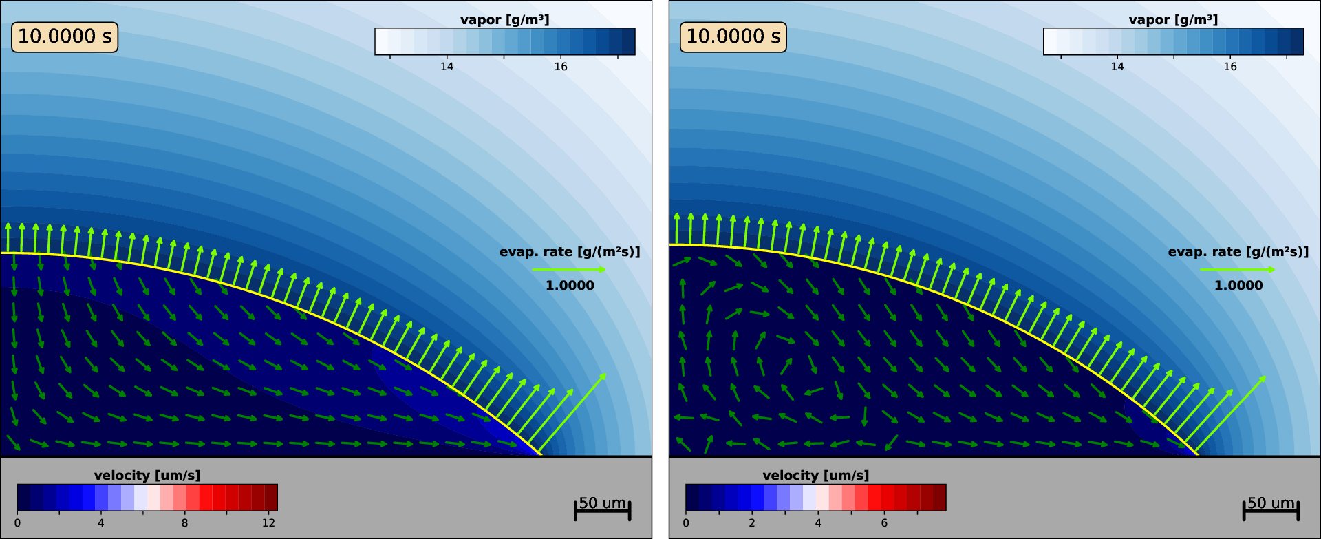
Fig. 7.6 Evaporating droplet with a pinned contact line (left) and with a constant contact angle (right).