7.1. Temperature conduction through two bodies of different conductivity
For a simple start, a static (i.e. non-moving) one-dimensional mesh consisting of two domains will be considered. The mesh should contain two interval domains "domainL" and "domainR", ranging from \(0\) to \(x_\text{I}\) and from \(x_\text{I}\) to \(L\) respectively, which are connected at a mutual interface "interface" at \(x_\text{I}\). We use the MeshTemplate class to provide such a mesh (cf. Section 4.3 for details):
from pyoomph import *
from pyoomph.equations.poisson import *

class TwoDomainMesh1d(MeshTemplate):
	def __init__(self,Ntot=100,xI=1,L=2,left_domain_name="domainA",right_domain_name="domainB"):
		super(TwoDomainMesh1d,self).__init__()
		self.Ntot, self.xI, self.L = Ntot, xI, L
		self.left_domain_name,self.right_domain_name=left_domain_name,right_domain_name

	def define_geometry(self):
		xI=self.nondim_size(self.xI)
		L=self.nondim_size(self.L)
		NA=round(self.Ntot*xI/L) # number of elements on domainA calculated from total number

		domainA=self.new_domain(self.left_domain_name)
		domainB=self.new_domain(self.right_domain_name)

		# Generate nodes
		nodesA=[self.add_node_unique(x) for x in numpy.linspace(0,xI,NA)]
		for x0,x1 in zip(nodesA, nodesA[1:]):
			domainA.add_line_1d_C1(x0,x1)	# and elements by pairs of nodes

		# same for domainB
		nodesB=[self.add_node_unique(x) for x in numpy.linspace(xI,L,self.Ntot-NA)]
		for x0,x1 in zip(nodesB, nodesB[1:]):
			domainB.add_line_1d_C1(x0,x1)

		# marking boundaries
		self.add_facet_to_boundary("left",[nodesA[0]])
		self.add_facet_to_boundary("interface",[nodesB[0]]) # coordsB[0] is actually = coordsA[-1]
		self.add_facet_to_boundary("right",[nodesB[-1]])
Note how we create two domains with the new_domain() calls and add line elements to both of these domains. During the latter, we use zip with a shifted node list to get the nodes in pairs, i.e. (node0,node1), (node1,node2), etc., to build the elements. It is important to note, since add_node_unique() will not create new nodes if a node is already existing at a point, that domainA[-1] is the very same node as domainB[0]. Thereby, this node, which is marked to be the interface "interface", is part of both domains.
Warning
If you want to couple the equations on different domains at mutual interfaces, all involved domains have to be generated within the very same MeshTemplate (or GmshTemplate). It is not possible to couple e.g. two LineMesh instances at an interface, not even if the position and the name of the interface are matching.
On the domains A and B, we want to solve the (nondimensional) temperature conduction equations, i.e. the Poisson equations
with the, in general different, thermal conductivities \(k_\text{A}\) and \(k_\text{B}\). The solution shall be subject to the boundary conditions \(T_\text{A}(0)=0\) and \(T_\text{B}(L)=1\). At the mutual interface "interface" at \(x_\text{I}\), we want to have a continuous temperature, i.e. \(T_\text{A}(x_\text{I})=T_\text{B}(x_\text{I})\). While the former boundary conditions can be realized by trivial DirichletBC, the latter requires some additional consideration, since it involves the temperature field on two different domains. We can write the boundary condition as a constraint with an associated Lagrange multiplier \(\lambda\) defined on the interface "interface". As usual, the constraint can be thought of as a minimization of the Lagrange multiplier contribution
with respect to \(\lambda\), \(T_\text{A}\) and \(T_\text{B}\). Let the corresponding test functions be \(\eta\), \(\Theta_\text{A}\) and \(\Theta_\text{B}\), then the corresponding weak terms read
In pyoomph, we can write again an InterfaceEquations class for this:
class ConnectTAtInterface(InterfaceEquations):
	def define_fields(self):
		self.define_scalar_field("lambda","C2") # Lagrange multiplier

	def define_residuals(self):
		my_field,my_test=var_and_test("T") # T on the domain where this InterfaceEquations object is attached to
		opp_field,opp_test=var_and_test("T",domain=self.get_opposite_side_of_interface()) # T on the interface, but evaluated in the opposite domain
		lagr,lagr_test=var_and_test("lambda") # Lagrange multiplier
		self.add_residual(weak(my_field-opp_field,lagr_test)) # constraint T_my-T_opp=0
		self.add_residual(weak(lagr,my_test)) # Lagrange Neumann contribution to the inside domain
		self.add_residual(weak(-lagr,opp_test)) # Lagrange Neumann contribution to the outside domain
We introduce again the Lagrange multiplier \(\lambda\) at the interface and add the weak contributions to the residuals. Later on, the ConnectTAtInterface object will be added to the "interface" of either "domainA" or "domainB", i.e. to @"domainA/interface" or @"domainB/interface". In both domains, we will have the temperature field var("T") defined. To distinguish between the fields on the inside (i.e. the domain where the ConnectAtInterface is attached to) and the outside (i.e. the opposite domain), we must use get_opposite_side_of_interface() for the domain to clearly state that we want to get the temperature of the opposite side of the interface, i.e. the temperature var("T") at the "interface", but evaluated at the opposite domain. Alternatively, we could have used var("T",domain="|.") as shortcut. It will also return the temperature field of the opposite side of the interface. To access the opposite bulk domain instead, use get_opposite_parent_domain() as domain or the shortcut var("T",domain="|..").
The driver code is quite trivial
class TwoDomainTemperatureConduction(Problem):
	def __init__(self):
		super(TwoDomainTemperatureConduction,self).__init__()
		self.conductivityA=0.5	# thermal conductivity of domain A
		self.conductivityB=2	# thermal conductivity of domain B

	def define_problem(self):
		self.add_mesh(TwoDomainMesh1d())

		# Assemble equations domainA
		eqsA=TextFileOutput()
		eqsA+=PoissonEquation(name="T",space="C2",coefficient=self.conductivityA,source=0)
		eqsA+=DirichletBC(T=0)@"left"

		# and equations of domainB
		eqsB=TextFileOutput()
		eqsB+=PoissonEquation(name="T",space="C2",coefficient=self.conductivityB,source=0)
		eqsB+=DirichletBC(T=1)@"right"

		# Interface connection. Must be added to one side of the interface, i.e. alternatively to eqsB
		eqsA+=ConnectTAtInterface()@"interface"

		self.add_equations(eqsA@"domainA")
		self.add_equations(eqsB@"domainB")


if __name__=="__main__":
	with TwoDomainTemperatureConduction() as problem:
		problem.solve()
		problem.output()
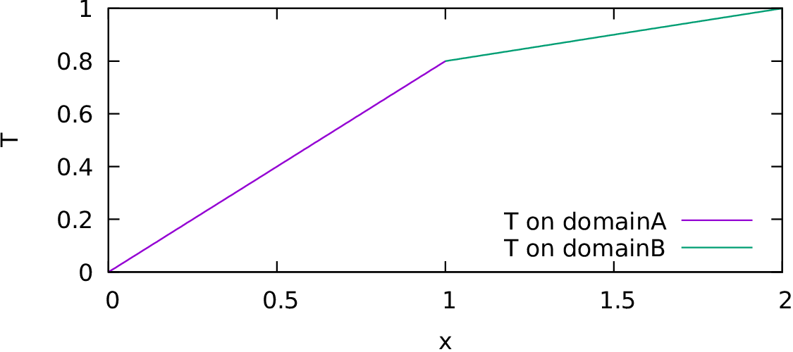
Fig. 7.1 Temperature conduction in two different domains with different conductivity, coupled at the mutual interface.
We add only one mesh, but assemble two Poisson equations, each with a different coefficient and with different DirichletBC terms. At the very end, the equations are restricted to "domainA" and "domainB", respectively. The ConnectTAtInterface can be either added to "domainA/interface" or "domainB/interface", but not on both simultaneously, since this would overconstrain the problem. The result is plotted in Fig. 7.1.
In terms of physics within this problem, we wonder, of course, whether the heat flux \(\vec{q}=-k\nabla T\) is indeed the same across the interface. Since the normals in "domainA" and "domainB" at the "interface" obey the relation \(\vec{n}_\text{A}=-\vec{n}_\text{B}\), a continuous heat flux would mean that
From the results in Fig. 7.1, we see that \(\partial_xT_\text{A}=0.8\) and \(\partial_xT_\text{B}=0.2\), and due to \(k_\text{A}=0.5\) and \(k_\text{B}=2\), it is indeed fulfilled. This is not just coincidence! From the weak form (7.1) of the enforced continuity of \(T\), we see that we impose \(\lambda\) as a Neumann flux to "domainA" and \(-\lambda\) to "domainB". The Neumann flux is exactly the heat flux and so continuity of this relation is actually a result of the enforcing. This also works, if the temperatures have a prescribed offset \(\Delta T\) in the enforcing, which would read
Hence, when enforcing continuity of fields across interfaces this way, one automatically gets the correct physics, here the continuity of the transported heat across the interface. However, (7.2) would be violated if the weak forms of the Poisson equations would be e.g. multiplied by a different factor in both domains, since this factor would also affect the Neumann term. Therefore, one has to pay attention.
Warning
Due to the above argument, one should not be tempted to set different scalings via set_scaling() of the Problem class or by the Scaling in dimensional problems. This can easily invalidate the continuity of the Neumann flux, which can lead to unphysical behavior. If one uses the same scale for non-dimensionalization of e.g. the temperature, e.g. by setting set_scaling(T=1*kelvin) at Problem level, this issue can be circumvented.
Note
It is cumbersome to write a coupling interface like the ConnectTAtInterface here for every field you want to connect at inter-domain interfaces. pyoomph already has the predefined class ConnectFieldsAtInterface, which allows enforcing continuity of scalar fields. In the current problem, we could just use ConnectFieldsAtInterface("T") instead of our custom class ConnectTAtInterface.