7.9.3. Full three dimensional implementation with wetting gradients on the substrate
Finally, we also want to use the droplet spreading case in three dimensions. Since equations are defined in a coordinate-system independent way within pyoomph, there is not much additional work required. The problem class reads
from droplet_spread_sliplength import * # Import the previous example
from pyoomph.meshes.simplemeshes import SphericalOctantMesh # import a 3d mesh, octant of a sphere

class DropletSpreading3d(Problem):
    def __init__(self):
        super(DropletSpreading3d, self).__init__()
        # The equilibirum contact angle will vary with the position along the substrate
        x,y=var(["coordinate_x","coordinate_y"])
        # some equilibrium contact angle expression
        self.contact_angle = (45+80*(minimum(x,2)-1)**2-30*(minimum(y,2)-1)**2) * degree

    def define_problem(self):
        # Eighth part of a sphere, rename the outer interface to "interface" and the z=0 plane to "substrate"
        mesh = SphericalOctantMesh(radius=1, interface_names={"shell":"interface","plane_z0":"substrate"})
        self.add_mesh(mesh)

        eqs = NavierStokesEquations(mass_density=0.01, dynamic_viscosity=1)  # flow
        # PseudoElasticMesh is a bit more expensive to calculate, but is more stable in terms of larger deformations than LaplaceSmoothedMesh
        eqs += PseudoElasticMesh()
        eqs += RefineToLevel(2)  # The SphericalOctantMesh only has four elements, so resolve it a bit
        # The shell of the SphericalOctantMesh carries a curved entity, so the nodes created by this
        # refinement land exactly on the sphere rather than on the polyhedron through the coarse
        # mesh's corners -- without it, the initial droplet would be short of its volume by 23%.

        # No flow through the boundaries and
        eqs += DirichletBC(mesh_x=0, velocity_x=0) @ "plane_x0"
        eqs += DirichletBC(mesh_y=0, velocity_y=0) @ "plane_y0"
        eqs += DirichletBC(mesh_z=0, velocity_z=0) @ "substrate"

        # free surface at the interface, equilibrium contact angle at the contact with the substrate
        n_free=var("normal",domain="domain/interface") # normal of the free surface
        n_substrate=vector(0,0,1) # normal of the substrate
        t_substrate=n_free-dot(n_free,n_substrate)*n_substrate # projection of the free surface normal on the substrate
        t_substrate=t_substrate/square_root(dot(t_substrate,t_substrate)) # normalized => tangent along the substrate locally outward
        N = cos(self.contact_angle)*t_substrate - sin(self.contact_angle)*n_substrate # Assemble N vector
        eqs += (FreeSurface(sigma=1) + EquilibriumContactAngle(N) @ "substrate") @ "interface"

        eqs += MeshFileOutput()  # output

        self.add_equations(eqs @ "domain")  # adding it to the system


if __name__ == "__main__":
    with DropletSpreading3d() as problem:
        # Gentler than the default 4x up / 0.25x down: an overshoot is expensive here (see the text)
        problem.DTSF_max_increase_factor = 1.25
        problem.DTSF_min_decrease_factor = 0.75
        problem.run(15, outstep=True, startstep=0.05,temporal_error=1,maxstep=2)
The equilibrium contact angle may be an arbitrary function of the coordinates. Here, we chose some expression that describes some wetting gradients along the substrate. As mesh, we use the SphericalOctantMesh, which is one eighth of a sphere. With only four elements, it has to be refined with a RefineToLevel to resolve the flow at all. Its shell is attached to a curved entity, so the nodes introduced by that refinement are placed exactly on the sphere instead of on the polyhedron spanned by the coarse mesh’s corners – otherwise the initial droplet would start out with 23% less volume than the sphere it is meant to be, no matter how far it is refined. However, three-dimensional ALE problems become easily very expensive in terms of computational costs. We get a high number of degrees of freedom for the velocity and also for the mesh position. Also, the motion of the mesh will couple with all equations and the Jacobian of the coupled system has quite a bunch of non-zero entries. Hence, one should not exaggerate the refinement level here. Instead of the LaplaceSmoothedMesh, now the predefined class PseudoElasticMesh is used. While both lead to a relaxation of a mesh that is subject to deformations due to the KinematicBC, the PseudoElasticMesh behaves as a deformable solid. This is often more stable, i.e. preventing strong deformations in a better way. It is, however, slightly more expensive to calculate than the LaplaceSmoothedMesh.
At the planar surfaces at \(x=0\), \(y=0\) and \(z=0\) of the mesh, we deactivate the mesh motion and the velocity in this direction to prevent any outflow through these domains. The tangential continuation of the free interface at the contact line \(\vec{N}\) is now more complicated than in two dimensions. We calculate it by first projecting the free surface normal \(\vec{n}\) on the normal \(\vec{n}_\text{s}=(0,0,1)\) of the substrate. This leads to a vector with zero \(z\)-component, i.e. oriented along the substrate plane and pointing outward from the contact line. When normalizing this vector \(\vec{t}_\text{s}\), we can assemble our vector by
The equilibrium contact angle \(\theta\) is a function of the local coordinates. \(\vec{t}_\text{s}\) depends on the local free surface. So in total, the contact line dynamics is really complicated and highly non-linear. Luckily, pyoomph does all the required internals, in particular the assembly of the analytical Jacobian, automatically.
In terms of implementation, one has to pay attention: It is important to use n_free=var("normal",domain="domain/interface"), whereas n_free=var("normal") would not work. n_free will be further evaluated at the contact line, not at the free surface. Hence, without domain specification, it would expand to the normal \(\vec{N}\) of the contact line, which is the tangential continuation of the free surface.
Since we are mostly interested in the final state of the droplet, we have not considered a slip length here, so that the droplet attains the equilibrium shape (cf. Fig. 7.12) as quickly as possible. Also the dynamic time stepping is beneficial for that. However, it is required to delimit the maximum time step with maxstep since too large steps lead to unacceptable errors in the volume conservation. The reason is due to the kinematic boundary condition, which is discrete in time.
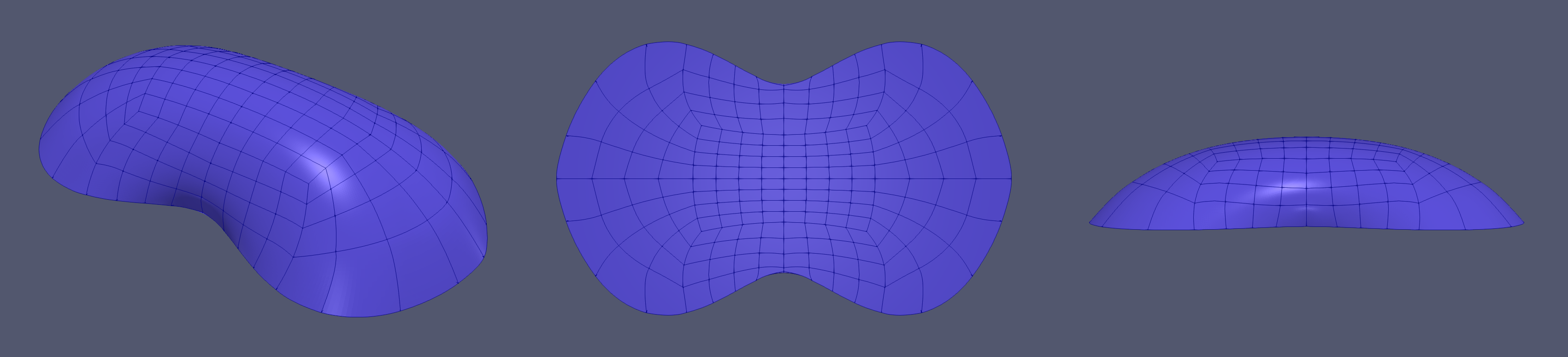
Fig. 7.12 Equilibrium shape of a three-dimensional droplet with varying equilibrium contact angle along the substrate.
Warning
Three-dimensional meshes and problems are currently still under development. Therefore, one should handle these with caution.