6.7.1. With free slip at the substrate
Similarly as done with lubrication theory in Section 5.4.2, we now want to let a droplet spread until it reaches its equilibrium contact angle. This time, however, we want to solve the full bulk flow including inertia and considering the full interface curvature. Hence, we use again the free surface equations from the previous example.
The key part to impose an equilibrium contact angle is the \([\cdot,\cdot]\) term in (6.7). It has not been considered so far, but it will become relevant now. This term can be added to boundaries of the free surface, i.e. to contact lines. The surface tension is fully balanced if \(\vec{N}\) is the outward pointing normal of the contact line, which is the outward pointing tangential continuation of the free interface at the boundaries. Let \(\theta\) be the equilibrium contact angle, then \(\vec{N}\) will read \((\cos(\theta),-\sin(\theta))\) if the droplet is at the equilibrium contact angle. Let us define the corresponding equation class that has to be added to the contact line to enforce this contact angle:
from free_surface import * # Load our free surface implementation
from pyoomph.meshes.simplemeshes import CircularMesh # Import a curved mesh


class EquilibriumContactAngle(InterfaceEquations):

	required_parent_type=DynamicBC # Must be attached to an interface with a DynamicBC

	def __init__(self,N):
		super(EquilibriumContactAngle,self).__init__()
		self.N=N # equilibrium vector

	def define_residuals(self):
		# get sigma from the DynamicBC object of the interface
		sigma=self.get_parent_equations().sigma
		# Contact line contribution
		v=testfunction("velocity")
		self.add_residual(-weak(sigma*self.N,v))
It is rather trivial, how \(-[\sigma\vec{N},\vec{v}]\) is implemented here. Note how we can access the free interface by accessing the DynamicBC equation of the parent domain, i.e. of the free surface, by get_parent_equations(). Since we have set required_parent_type=DynamicBC, pyoomph knows that get_parent_equations() should give the DynamicBC and not the KinematicBC contribution. Only the former has the surface tension property sigma defined.
The problem class itself is very similar to the previous example:
class DropletSpreadingProblem(Problem):
	def __init__(self):
		super(DropletSpreadingProblem,self).__init__()
		self.contact_angle=45*degree # equilibrium contact angle

	def define_problem(self):
		# hemi-circle mesh, i.e. initial contact angle of 90 degree, free interface "interface", symmetry axis "axis" and bottom interface "substrate"
		mesh=CircularMesh(radius=1,segments=["NE"],straight_interface_name={"center_to_north":"axis","center_to_east":"substrate"},outer_interface="interface")
		self.add_mesh(mesh)

		self.set_coordinate_system("axisymmetric") # axisymmetry

		eqs=NavierStokesEquations(mass_density=0.01,dynamic_viscosity=1) # flow
		eqs+=LaplaceSmoothedMesh() # Laplace smoothed mesh
		eqs+=RefineToLevel(4) # refine, since the CircularMesh is coarse by default
		eqs+=DirichletBC(mesh_x=0,velocity_x=0)@"axis" # fix mesh x-position, no flow through the axis
		eqs+=DirichletBC(mesh_y=0,velocity_y=0)@"substrate" # fix substrate at y=0, no flow through the substrate
		# free surface at the interface, equilibrium contact angle at the contact with the substrate
		N=vector(cos(self.contact_angle),-sin(self.contact_angle))
		eqs+=(FreeSurface(sigma=1)+EquilibriumContactAngle(N)@"substrate")@"interface"
		eqs+=MeshFileOutput() # output

		self.add_equations(eqs@"domain") # adding it to the system


if __name__=="__main__":
	with DropletSpreadingProblem() as problem:
		problem.run(50,outstep=True,startstep=0.25)
Important differences are the mesh, which is now the north-east ("NE") quarter of a CircularMesh with renamed boundaries and a suitable RefineToLevel by thereof, the selection of an "axisymmetric" coordinate system and the fact that now both \(x\) and \(y\) mesh coordinates are allowed to move. We set the \(x\)-coordinate (i.e. the \(r\)-coordinate) of the mesh and the \(x\)-velocity (\(r\)-velocity) to zero at the axis of symmetry and likewise the \(y\)-coordinate and \(y\)-velocity to zero at the substrate. Note that the \(x\)-velocity at the substrate is completely free, i.e. it corresponds to an (unrealistic) free slip boundary at the moment. This can be seen on the left side of Fig. 6.7. The droplet spreads quickly and the fluid can flow unhindered tangentially along the substrate.
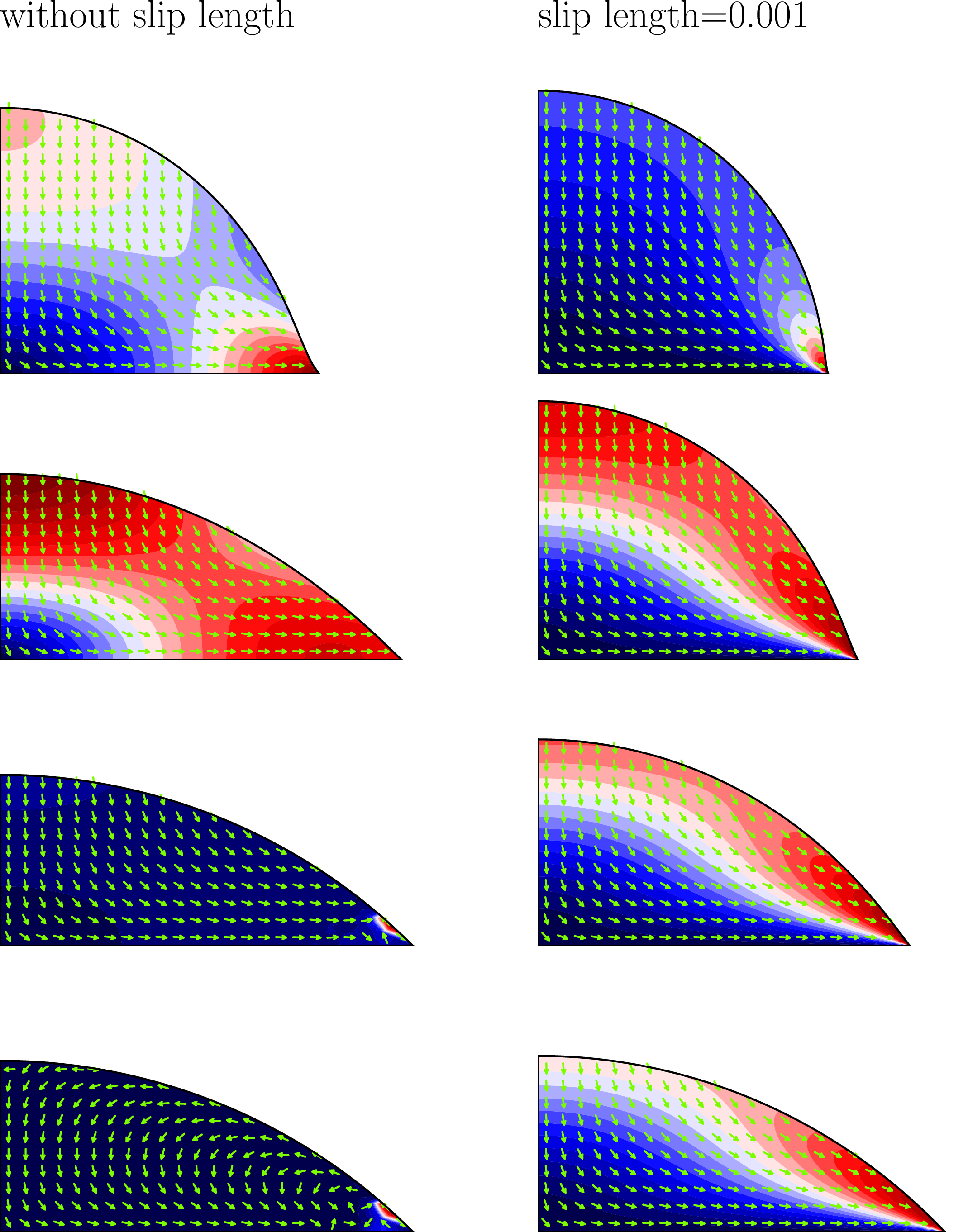
Fig. 6.7 (left) Spreading with free slip at the substrate. (right) Spreading with a tiny slip length.