10.4.2. Rayleigh-Plateau instability in presence of a substrate

The previous example was quite simple. In particular, the calculation of the dispersion relation could also have been done analyically by pen and paper. However, the stability analysis in an additional Cartesian direction can be used to quickly investigate considerably more intricate problems.

Here, we want to consider a long printed line of a liquid on a substrate, also called rivulet. We assume that this rivulet is infinitely long in the \(z\)-direction and its shape is independent on \(z\). Alternatively, we can also think of a such a rivulet confined between two plates with distance \(L=2\pi/k\), free slip conditions and an \(90^\circ\) equilibrium contact angle with respect to the plate tangent.

In absence of a substrate, i.e. for a cylindrically shaped liquid bridge, it is well-known that it undergoes a Rayleigh-Plateau instability when \(L/R>2\pi\). However, how does the dynamics change if we consider a rivulet on a substrate instead? Of course, there must be a specific length (or wavenumber \(k\) in \(z\)-direction) when this printed line also undergoes a Rayleigh-Plateau instability, provided that we allow for some slip at the substrate. However, how does the critical wavenumber \(k\) and the time scale of the instability depend on e.g. the contact angle with respect to the substrate and/or the slip length at the substrate?

We can easily find all the answers by expressing the shape of base solution only in the \(x\)-\(y\)-plane and let pyoomph calculate the stability of such a solution with respect to perturbations in the third direction \(z\). We will use Stokes flow for the liquid and combine it with a moving mesh to allow for shape deformations. Moreover, we only consider the right half (i.e. \(x\geq 0\)) and thereby only selects modes which are symmetric with respect to \(x\) in the following. Therefore, our mesh just creates half of the domain:

class RivuletMesh(GmshTemplate):
    def define_geometry(self):
        self.default_resolution=0.1
        self.mesh_mode="tris"
        cl_factor=0.5 # Make it finer at the contact line
        pr=cast(RivuletProblem,self.get_problem())
        geom=DropletGeometry(volume=pi/2,rivulet_instead=True,contact_angle=pr.theta)
        p00=self.point(0,0)
        prl=self.point(-geom.base_radius,0,size=cl_factor*self.default_resolution) # Mirrored point for the circle_arc
        prr=self.point(geom.base_radius,0,size=cl_factor*self.default_resolution) # contact line
        p0h=self.point(0,geom.apex_height) # Top of the droplet

        self.circle_arc(prr,p0h,through_point=prl,name="interface")
        self.line(prr,p00,name="substrate")

        self.line(p00,p0h,name="axis")
        self.plane_surface("interface","substrate","axis",name="liquid")

Note how we use DropletGeometry with the kwarg rivulet_instead=True to convert the volume and the contact angle (which we obtain from the problem defined later on) to the base radius and apex height. Using rivulet_instead=True actually converts the value shipped by volume as surface area of the circle segment. In particular, using the volume of \(\pi/2\), it gives a radius of curvature of unity for a contact angle \(\theta=90^\circ\).

For the problem class, we just define the two parameters (slip length and contact angle) and add all equations to the system. Since we will have an effectively three-dimensional dimensional problem, it is important again to pass the wall_tangent to the NavierStokesContactAngle. This is a vector pointing inward to the bulk domain tangentially along the substrate, i.e. orthogonal to the wall_normal which is just the axially upward pointing normal. In a pure axisymmetric or 2d Cartesian case wall_tangent=vector(-1,0) is fine, but it is not true once the free surface deforms in a third direction (cf. Section 6.6.3). If again \(\vec{n}\) is the normal of the free surface and \(\vec{n}_\mathrm{w}\) is the wall normal, we can use the double cross product \(\vec{n}_\mathrm{w}\times(\vec{n}_\mathrm{w}\times \vec{n})\) to obtain such a (non-normalized) vector. We can use the known bac-cab identity along with \(\|\vec{n}_\mathrm{w}\|=1\) to calculate it via \(\vec{n}_\mathrm{w}(\vec{n}_\mathrm{w}\cdot\vec{n})-\vec{n}\) and subsequently normalize the result, which is valid for all contact angles \(0<\theta<180^\circ\).

class RivuletProblem(Problem):
    def __init__(self):
        super().__init__()
        # Contact angle and slip length
        self.theta,self.sliplength=self.define_global_parameter(theta=90*degree,sliplength=1)

    def define_problem(self):
        self+=RivuletMesh() # Add a 2d mesh

        # Assemble the equation system
        eqs=HyperelasticSmoothedMesh() # Moving mesh, Hyperelastic mesh is quite robust, since we do not remesh in this particular tutorial
        eqs+=NavierStokesEquations(dynamic_viscosity=1) # bulk flow
        # Boundary conditions:
        # Navier-slip and no penetration at the substrate
        eqs+=( NavierStokesSlipLength(sliplength=self.sliplength) + DirichletBC(velocity_y=0,mesh_y=0) )@"substrate"
        # Free surface at the interface
        eqs+=NavierStokesFreeSurface(surface_tension=1)@"interface"
        # Impose a contact angle at the contact line
        wall_normal=vector(0,1,0) # The substrate has an upwards normal (to be read as 0*e_r+1*e_z+0*e_phi)
        ninter=var("normal",domain="..") # The normal at the free surface (one domain up when evaluated at the contact line)
        wall_tangent=wall_normal*dot(wall_normal,ninter)-ninter # double cross product bac-cab rule (with dot(wall_normal,wall_normal)=1)
        wall_tangent=wall_tangent/square_root(dot(wall_tangent,wall_tangent)) # Normalize it
        eqs+=NavierStokesContactAngle(contact_angle=self.theta,wall_normal=wall_normal,wall_tangent=wall_tangent)@"interface/substrate"
        # Symmetry at the axis
        eqs+=DirichletBC(mesh_x=0,velocity_x=0)@"axis"
        # Enforce the volume/area of the liquid by a pressure constraint
        eqs+=EnforceVolumeByPressure(volume=pi/4)

        eqs+=MeshFileOutput()
         # Apply the equation system to the liquid domain
        self+=eqs@"liquid"

This only sets up the two-dimensional problem. The eigenanalysis with the additional normal mode is activated in the driver code:

problem=RivuletProblem() # Create the problem
# Setup the problem for k-stability analysis, we do not need an analytic Hessian, since we don't do any bifurcation tracking
problem.setup_for_stability_analysis(additional_cartesian_mode=True,analytic_hessian=False)
# Use the SLEPc eigensolver with MUMPS
problem.set_eigensolver("slepc").use_mumps()
problem.solve() # Solve the base state
problem.save_state("start.dump") # Save the start case at 90°


# Scan the contact angle
for theta_deg in [60,90,120]:
    problem.load_state("start.dump",ignore_outstep=True)
    problem.go_to_param(theta=theta_deg*degree)
    # Scan the slip length (either essentially free slip or quite low slip length)
    for sl in [10000,0.01]:
        problem.go_to_param(sliplength=sl)

        outf=problem.create_text_file_output("for_"+str(round(float(problem.theta/degree)))+"_deg_SL_"+str(sl)+".txt",header=["k","Lambda"])

        for k in numpy.linspace(0.01,1.5,50):
            problem.solve_eigenproblem(1,normal_mode_k=k) # Solve the k-dependent eigenproblem
            evs=problem.get_last_eigenvalues()
            outf.add_row(k,numpy.real(evs[0]))

Again, it just takes the call of setup_for_stability_analysis() with additional_cartesian_mode=True to activate this feature and shipping normal_mode_k=k to the call of solve_eigenproblem().

The eigenvalues are plotted in Fig. 10.8. It is apparent that, indepedently of the slip length, the critical wavenumber is at \(k=1\) for \(\theta=90^\circ\), which is reasonable, since the problem can be essentially mirrored at both axis to get the conventional Rayleigh-Plateu instability (at least for high slip lengths). A smaller slip influences the magnitude of the eigenvalues, which is reasonable, since it damps the motion of the contact line. For other contact angles, it is essentially the same, but the cricial wave number shifts. Due to the fixed cross-sectional area of the rivulet, a change in contact angle influences the radius of curvature, therefore the critical wave number shifts. Some plots of the eigendynamics are shown in Fig. 10.9, from which the influence of the slip length is clearly apparent.

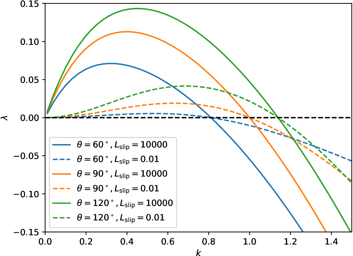
Fig. 10.8 Eigenvalues of the rivulet with different contact angles and slip lengths plotted against the wave number \(k\).

To visualize the eigenmodes, it is beneficial to modify the problem code above by adding some operators to the MeshFileOutput:

from pyoomph.meshes.meshdatacache import MeshDataCombineWithEigenfunction,MeshDataCartesianExtrusion
eqs+=MeshFileOutput(operator=MeshDataCombineWithEigenfunction(0)+MeshDataCartesianExtrusion(50))

Here MeshDataCombineWithEigenfunction will combine the base state with the eigenfunction at index 0, so that both the base solution and the eigenfunction are written to the file for Paraview. MeshDataCartesianExtrusion will apply the extrusion in the \(z\)-direction, respecting the oscillation of the eigenmode with \(\exp(ikz)\). To write this output, add the output() method of the Problem to the driver code where you want to have output, however, after an solve_eigenproblem(), so that the eigensolution is available. Afterwards, you can load the files in Paraview, use the Calculator filter with an expression iHat*Eigen_coordinate_x+jHat*Eigen_coordinate_y to cast the mesh perturbation to a vector, combine it with Wrap by Vector and Reflect filters and you obtain plots like shown in Fig. 10.9.

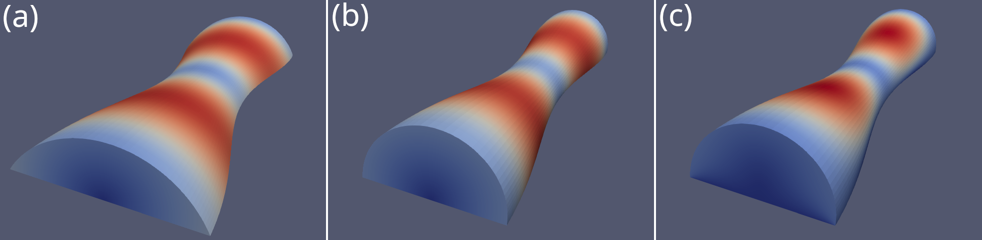
Fig. 10.9 Eigendynamics at \(k=0.6\) of the rivulet with (a) \(\theta=60^\circ, L_\mathrm{slip}=10000\), (b) \(\theta=90^\circ, L_\mathrm{slip}=10000\) and (c) \(\theta=90^\circ, L_\mathrm{slip}=0.01\). Color-coded is the velocity magnitude.

Download this example

Download all examples