10.5. Continuation of eigenbranches
While solve_eigenproblem() can solve for eigenvalues, it is sometimes hard to order them when varying a parameter. All eigenvalues can change, cross each other and it is then cumbersome to disentangle what is happening to each eigenbranch. Similar to bifurcation tracking, it is also possible to track a specific eigenfunction. To that end, we first have to solve for an eigenvalue/-vector pair as an initial guess. Then, we solve an augmented system for the base state and this particular eigenvalue/-vector pair. Upon continuation, we will follow this particular eigenbranch.
We will discuss this feature on the basis of a liquid bridge with gravity. In the absence of gravity, it is well known that the system undergoes a Rayleigh-Plateau instability at \(L/R=2\pi\). But what happens if we add gravity in the axial direction to the system? Since the Rayleigh-Plateau instability sets in at rest, we will ignore the inertia term, i.e. going for Stokes flow. The problem class is quite simple and reads:
class LiquidBridgeProblem(Problem):
    def __init__(self):
        super().__init__()
        # Length of the domain
        self.L=self.define_global_parameter(L=2*pi)
        self.Bo=self.define_global_parameter(Bo=0)
        self.R=1 # Radius of the cylinder
        self.Nr=6 # Number of elements in the radial direction

    def define_problem(self):
        # Axisymmetric problem
        self.set_coordinate_system("axisymmetric")

        # Calculate the number of elements in the axial direction
        aspect0=float(self.L/self.R)
        Nl=round(aspect0*self.Nr)

        # Add the mesh
        self+=RectangularQuadMesh(size=[self.R,self.L],N=[self.Nr,Nl])

        # Bulk equations are: Stokes equations, pseudo-elastic mesh, mesh file output
        eqs=StokesEquations(dynamic_viscosity=1,bulkforce=self.Bo*vector(0,-1))
        eqs+=PseudoElasticMesh()
        eqs+=MeshFileOutput(operator=MeshDataCombineWithEigenfunction(0)) # Add also the zeroth eigenfunction to the output

        # Boundary conditions: Axisymmetry, no-slip at the bottom, no-slip at the top, no-slip at the right, free surface at the left
        eqs+=AxisymmetryBC()@"left"
        eqs+=DirichletBC(velocity_x=0,velocity_y=0,mesh_y=0,mesh_x=True)@"bottom"
        eqs+=DirichletBC(velocity_x=0,velocity_y=0,mesh_x=True)@"top"
        # However, since we want to vary the length, we must trick a bit
        # First, we enforce that mesh_y=L at the top (i.e. we adjust mesh_y so that var("mesh_y")-self.L=0)
        eqs+=EnforcedDirichlet(mesh_y=self.L)@"top"
        # However, thereby, the Lagrange multiplier for the kinematic boundary condition is not automatically pinned to zero
        # Since mesh_y is a degree of freedom now at the right/top corner, the kinematic BC constraint is not pinned automatically
        # So we must pin it manually
        eqs+=DirichletBC(_kin_bc=0)@"right/top"

        # Free surface at the left
        eqs+=NavierStokesFreeSurface(surface_tension=1)@"right"

        # Volume constraint for the pressure to fix the volume
        Vdest=pi*self.R**2*self.L
        P,Ptest=self.add_global_dof("P",equation_contribution=-Vdest) # Subtract the desired volume
        eqs+=WeakContribution(1,Ptest) # Integrate the actually present volume, P is now determined by V_act-V_desired=0
        #eqs+=WeakContribution(P,"pressure") # And this pressure is added to the pressure field
        eqs+=AverageConstraint(_kin_bc=P)@"right" # Average the normal traction to agree with the gas pressure

        # Add the equations to the problem
        self+=eqs@"domain"
Note how we fix the top of the domain to the parameter \(L\) via an EnforcedDirichlet. Unlike a conventional DirichletBC, the mesh_y positions are now still degrees of freedom of the system, but enforced via Lagrange multipliers to \(L\). This helps for continuation in \(L\), since the mesh positions are now considered in the arclength tangent as well. However, since the axial mesh position at the contact line is now a degree of freedom, pyoomph does not automatically pin the Lagrange multiplier for the kinematic boundary condition (see Section 6.5, where we pin the Lagrange multiplier of the kinematic boundary condition only if all mesh positions are pinned). Therefore, we manually have to pin it, since the system is otherwise overconstrained.
The volume is again enforced by varying the gas pressure, which is added as normal traction by enforcing the average of the kinematic boundary condition Lagrange multipliers (which are normal tractions) to the gas pressure.
Once set up, we can use this problem and solve for the stationary state at the minimum considered length \(L\). We store this state, so that we can load it after each branch. To scan an eigenbranch, we first load the start point, solve the eigenproblem for the initial guess and then activate eigenbranch tracking with the desired index of the eigenvalue. By continuation of the length, we can follow this particular eigensolution. At the end of the scan for \(\mathrm{Bo}=0\), we again store the base solution. This is then used as a start for other branches with \(\mathrm{Bo}\neq 0\). As you can see in the figure below, the presence of gravity leads to a fold bifurcation before the conventional Rayleigh-Plateau instability actually happens. With our approach, we find the other eigenbranches easily.
with LiquidBridgeProblem() as problem:

    # Generate analytically derived C code for the Hessian (for the eigenbranch tracking)
    problem.setup_for_stability_analysis(analytic_hessian=True)
    problem.set_c_compiler("system").optimize_for_max_speed()
    # Solve the base problem
    problem.solve()
    L0=float(problem.L) # Store the initial length
    minL=0.8*L0
    maxL=1.2*L0
    problem.go_to_param(L=minL) # Go to the stable length
    problem.save_state("start.dump") # Save the initial state

    neigen=2
    def create_Bond_curve(Bo,eigenindex,startfile, postfix,start_high_L=False):
        problem.load_state(startfile,ignore_outstep=True) # Load the initial state
        # Go to the desired Bond number and length
        problem.go_to_param(Bo=Bo)
        problem.go_to_param(L=(maxL if start_high_L else minL))
        # Create and output file for this Bond number
        curve=NumericalTextOutputFile(problem.get_output_directory("curve_Bo_"+str(Bo)+"_"+str(eigenindex)+"_"+postfix+".txt"),header=["L","ReLambda","ImLambda"])
        # Solve the eigenproblem and add the first eigenvalue to the curve
        problem.solve_eigenproblem(neigen)
        # We need to solve one eigenproblem only
        # Now we activate eigenbranch tracking
        problem.activate_eigenbranch_tracking(eigenvector=eigenindex)
        problem.solve() # And solve for it

        # Scan the curve
        curve.add_row(problem.L,numpy.real(problem.get_last_eigenvalues()[0]),numpy.imag(problem.get_last_eigenvalues()[0]))
        dL0=(maxL-minL)/20*(-1 if start_high_L else 1) # Initial step size
        dL=dL0 # Current step size
        while problem.L.value<=maxL and problem.L.value>=minL:
            # We must use arclength continuation here, since we hit fold bifurcations if Bo!=0
            dL=problem.arclength_continuation("L",dL,max_ds=dL0)
            curve.add_row(problem.L,numpy.real(problem.get_last_eigenvalues()[0]),numpy.imag(problem.get_last_eigenvalues()[0]))
        problem.deactivate_bifurcation_tracking() # Stop the bifurcation tracking (here, eigenbranch tracking)


    # Create the Bond curve for Bo=0
    create_Bond_curve(0,0,"start.dump","std")
    # Save the end state for later (high L)
    problem.save_state("end.dump")
    # Create the Bond curve for Bo=1
    create_Bond_curve(0,1,"start.dump","std")

    # Now create the lower L curves for Bo=0.0025
    create_Bond_curve(0.0025,0,"start.dump","fold")
    create_Bond_curve(0.0025,1,"start.dump","fold")

    # And also the higher L curves for Bo=0.0025
    create_Bond_curve(0.0025,0,"end.dump","unstab",start_high_L=True)
    # Save the end state for later, when going back to Bo=0
    problem.save_state("end2.dump")
    create_Bond_curve(0.0025,1,"end.dump","unstab",start_high_L=True)

    # Now we have found a rather strange unstable branch, where the interface is not straight despite of Bo=0.
    # Here, the two curvatures cancel each other out, but it is not stable.
    create_Bond_curve(0,0,"end2.dump","unstab")
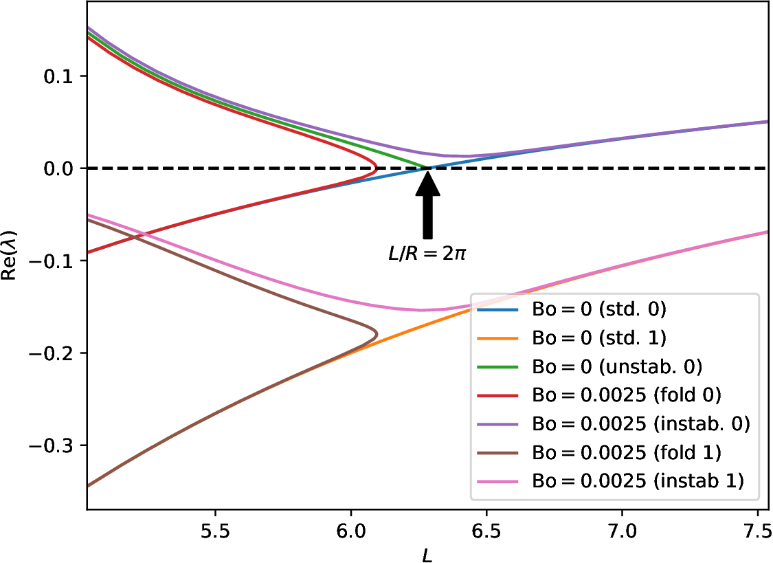
Fig. 10.10 Eigenbranches of a liquid bridge with gravity. The original Rayleigh-Plateau instability is broken by the presence of gravity. The subcritical pitchfork bifurcation becomes imperfect when gravity is considered.
Note
If you want to find the pitchfork bifurcation using the bifurcation tracking tools (cf. Section 3.11.7), you will get some issues here. Since the symmetry broken by the pitchfork bifurcation is not centered around the \(x\)-axis, the pitchfork won’t be found. To overcome this issue, you can just enforce the "top" boundary to be at mesh_y=self.L/2 and do it the same way with the "bottom" to mesh_y=-self.L/2 with an EnforcedDirichlet including the pinning of the _kinbc at "right/bottom". If the symmetry broken by the pitchfork is symmetric with respect to the \(x\)-axis, it works fine.