10.4.1. Numerically obtaining the dispersion relation of a Turing instability
The additional Cartesian mode can be even used if \(N=0\) holds, i.e. we can expand a single point to an interval of length \([0:2\pi/k)\) (with periodic boundary conditions) and determine the eigenvalues and eigenfunctions here. This allows us to quickly scan over \(k\) to numerically extract a dispersion relation. We will discuss this here for a simple Turing instability (see [26, 42, 47] for more details).
We begin by the equation class, which takes the diffusivity ratio and the reaction terms of the activator and inhibitor as arguments:
class TuringEquations(Equations):
    def __init__(self,d,f,g):
        super().__init__()
        self.d=d # Diffusivity ratio
        self.f,self.g=f,g # Reaction terms

    def define_fields(self):
        self.define_scalar_field("u","C2") # activator
        self.define_scalar_field("v","C2") # inhibitor

    def define_residuals(self):
        u,utest=var_and_test("u")
        v,vtest=var_and_test("v")
        self.add_weak(partial_t(u)-self.f,utest).add_weak(grad(u),grad(utest))
        self.add_weak(partial_t(v)-self.g,vtest).add_weak(self.d*grad(v),grad(vtest))
The problem class now just defines the reaction terms according to the Gierer-Meinhardt model [26, 42]. We then add a PointMesh, which is a \(0\)-dimensional mesh consisting only of a single point and define the just developed equations on this mesh. Of course, on such a mesh, we could only get the eigendynamics of the ODEs \(\dot u=f, \dot v=g\), arising in absence of the diffusion terms. However, we will soon use the additional Cartesian normal mode to add a single \(x\)-coordinate to quickly and exactly (i.e. without any spatial discretization) calculate the eigenvalues of the corresponding one-dimensional system, i.e. with diffusion terms.
class TuringProblem(Problem):
    def __init__(self):
        super().__init__()
        # Parameters, see https://dx.doi.org/10.1007/s10994-023-06334-9
        self.d,self.a,self.b,self.c=self.define_global_parameter(d=40,a=0.01,b=1.2,c = 0.7)
        # Reaction terms
        self.f=self.a-self.b*var("u")+var("u")**2/(var("v")*(1+self.c*var("u")**2))
        self.g=var("u")**2-var("v")

    def define_problem(self):
        # We add a 0d mesh here. So we do not have any spatial information
        from pyoomph.meshes.simplemeshes import PointMesh
        self+=PointMesh()
        eqs=TuringEquations(self.d,self.f,self.g)
        # Some reasonable guess here (not the exact solution)
        eqs+=InitialCondition(u=(self.a + 1)/self.b, v=(self.a + 1)**2/self.b**2)
        self+=eqs@"domain"
In the driver code, we call setup_for_stability_analysis() with additional_cartesian_mode=True to add the additional Cartesian normal mode. Supplying normal_mode_k=k during the calls of solve_eigenproblem() will select the wavenumber \(k\) for such a one-dimensional case.
We can thereby quickly scan the full dispersion relation:
    with TuringProblem() as problem:
        # Take a quick C compiler, to speed up the code generation
        problem.set_c_compiler("tcc")
        # Important part: This will add the N+1 dimension allowing for perturbations like exp(i*k*x+lambda*t)
        problem.setup_for_stability_analysis(additional_cartesian_mode=True)
        # Solve for the flat stationary solution
        problem.solve()
        # And scan over the k values, solve the normal mode eigenvalue problem and write the results to a file
        output=problem.create_text_file_output("dispersion.txt",header=["k","ReLamba1","ReLambda2","ImLambda1","ImLambda2"])
        for k in numpy.linspace(0,1,400):
            problem.solve_eigenproblem(2,normal_mode_k=k)
            evs=problem.get_last_eigenvalues()
            output.add_row(k,numpy.real(evs[0]),numpy.real(evs[1]),numpy.imag(evs[0]),numpy.imag(evs[1]))
Of course, the results depicted in Fig. 10.6 can also be calculated analytically. However, it is already rather complicated to find the stationary base solution. Also, it is only a few lines of code and we have already implemented our equation class to be used in arbitrary dimensions and coordinate systems.
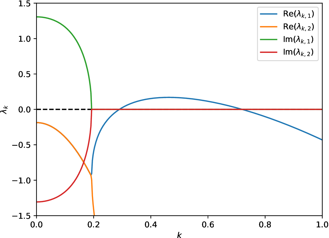
Fig. 10.6 Numerically calculated dispersion relation of the Turing instability.
In particular, we can quickly get a good guess for the dominant wavenumber, here around \(k=0.46\). This can be used to estimate a reasonable domain size for e.g. a two-dimensional transient simulation, where we can reuse the existing equation and problem class to obtain Turing patterns as depicted in Fig. 10.7. The corresponding script can be found here: turing_transient.py.
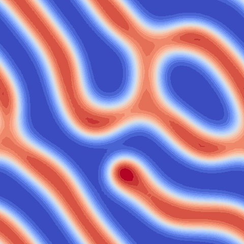
Fig. 10.7 After finding the dominant wave number, we can run transient 2d simulations with a suitable domain size.