3.10.2. Playing tennis in pyoomph - custom expression with dimensions
The next problem will be a bit more comprehensive and it will involve several techniques we have learned so far, namely using physical dimensions, custom math expressions and temporal adaptivity. We want to simulate a simple tennis match. As in all physics exams, there is no air friction acting on the ball, the problem is one-dimensional and the tennis rackets behave as a Hookean spring, but only if the position of the ball exceeds the position of the racket. Mathematically, we solve
where \(F_1\) and \(F_2\) are the forces of the rackets, which take action whenever the ball reaches the positions \(X_1\) and \(X_2\) of the rackets:
For these forces, we write our CustomMathExpression in python, however, now taking the positions in meters and resulting in a dimensional force with the unit \(\:\mathrm{N}\):
from pyoomph import *
from pyoomph.expressions import *
from pyoomph.expressions.units import *

# Force of a tennis racket as function of the ball position and the racket position
# This will create a function Force(ball_position,racket_position)
# Both positions must have the unit of meter
# And the result is a force measured in Newton
class TennisRacket(CustomMathExpression):
    def __init__(self,*,direction=1,spring_constant=1000*newton/meter):
        super(TennisRacket, self).__init__()
        self.direction=direction # sign of the force
        # Store a non-dimensional value of the spring constant
        self.k_in_N_per_m=float(spring_constant/(newton/meter))

    # Input arguments are converted to numerical values by treating the input as meter (for both arguments, ball and racket position)
    def get_argument_unit(self,index:int):
        return meter # return meter, no matter whether index==0 or index==1

    # The result is obtained by multiplying the result of 'eval' by newton
    def get_result_unit(self):
        return newton

    # This routine is now entirely nondimensional
    def eval(self,arg_array):
        # get the input values (numerical float values!)
        ball_pos_in_m=arg_array[0] # measured int meter
        racket_pos_in_m=arg_array[1] # measured int meter
        # calculate the distance (also in meter)
        distance_in_m=self.direction*(ball_pos_in_m-racket_pos_in_m)
        if distance_in_m>=0: # in front of the racket
            return 0.0 # numerical float value of the force [in newton]
        else:
            # Force of the racket on the ball
            force_in_newton=-self.direction*self.k_in_N_per_m*distance_in_m
            return force_in_newton # result is treated in newton
To allow for arguments with physical units as input arguments, we must implement the function get_argument_unit(), which returns the unit used for non-dimensionalization of the input arguments. The argument index here can be used to identify which argument to the custom math function is meant. Furthermore, the result of our calculation, i.e. of the force \(F_1\) and \(F_2\) shall be measured in \(\:\mathrm{N}\), which we tell pyoomph by implementing the method get_result_unit(). Everything else, i.e. the entire calculation of the force will now be done by float numbers in Python. The values stored in arg_array are float numbers giving the position of the ball and the position of the racket in meters. The return value of eval must also be a float, which is eventually multiplied by the result of get_result_unit(), i.e. by \(\:\mathrm{N}\), to give a dimensional force.
The class for the equation for the ball position \(x\) is again trivial:
class NewtonsLaw1d(ODEEquations):
    def __init__(self,mass,force):
        super(NewtonsLaw1d, self).__init__()
        self.mass=mass
        self.force=force

    def define_fields(self):
        # bind the scale factors (defined on problem level)
        T=scale_factor("temporal")
        X=scale_factor("spatial")
        # we set the scales as well as the test function scales here locally in the equation class
        self.define_ode_variable("x",scale=X,testscale=T**2/X) # same test scale as in the dimensional harmonic oscillator before
        self.define_ode_variable("xdot",scale=X/T,testscale=T/X) # velocity scales as X/T, test scale T/X will cancel this out

    def define_residuals(self):
        x,xdot=var(["x","xdot"])
        residual=(partial_t(xdot)-self.force/self.mass)*testfunction(x)
        residual+=(partial_t(x)-xdot)*testfunction(xdot)
        self.add_residual(residual)
Differently than before, we define not only the test function scales in the define_fields() method, but also the scales themselves by adding the argument scale to the define_ode_variable(). The position \(x\) will be nondimensionalized by a scale "spatial", which will be set later. The velocity \(\dot x\), i.e. xdot, is nondimensionalized by "spatial"/"temporal", which is a reasonable choice for a velocity. The test scales are again chosen in such a way that all physical units cancel out in the added residual. Both missing scales "spatial" and "temporal" are set at problem level using set_scaling().
class TennisProblem(Problem):
    def __init__(self):
        super(TennisProblem, self).__init__()
        self.top_racket_force=TennisRacket(direction=-1,spring_constant=5*newton/meter)
        self.bottom_racket_force=TennisRacket(direction=1,spring_constant=20*newton/meter)
        self.top_position=10*meter
        self.bottom_position=-10*meter
        self.ball_mass=60*gram
        self.ball_pos0=0*meter
        self.ball_velo0=10*meter/second

    def define_problem(self):
        self.set_scaling(spatial=1*meter,temporal=1*second)
        ball_pos=var("x")
        racket_force=self.top_racket_force(ball_pos,self.top_position)
        racket_force+=self.bottom_racket_force(ball_pos,self.bottom_position)
        racket_force=subexpression(racket_force)

        ball_eq=NewtonsLaw1d(mass=self.ball_mass,force=racket_force)
        ball_eq+=InitialCondition(x=self.ball_pos0,xdot=self.ball_velo0)
        ball_eq += ODEObservables(top_position_in_m=self.top_position/meter,bottom_position_in_m=self.bottom_position/meter)
        ball_eq+=ODEFileOutput()
        ball_eq+=TemporalErrorEstimator(x=1,xdot=1)

        self.add_equations(ball_eq@"ball")

if __name__=="__main__":
    with TennisProblem() as problem:
        problem.run(endtime=20*second,outstep=True,temporal_error=0.0025,startstep=0.01*second)
In the constructor, we initialize two rackets, one at the top and one at the bottom with different values for the spring constant \(k\). Thereby, we provide the two functions that calculate the force of the racket as function of the ball position and the racket position. In the define_problem() method, first the scalings "spatial" and "temporal" are set at problem level. The former is then used for the scale of "x" and the quotient of both is used for "xdot" at equation level. Then, the equation of motion, NewtonsLaw1d is constructed, with a force consisting the sum of both racket forces. Again, it is encapsulated in a subexpression() as recommended for additional computation speed. The remainder is trivial, but note that again a TemporalErrorEstimator is added to monitor the error made by the adaptive time stepping.
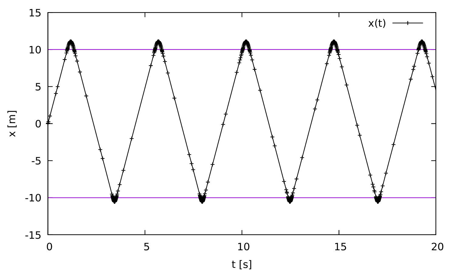
Fig. 3.10 Tennis with pyoomph. One clearly sees how the dynamic time stepping kicks in when the forces of the rackets are acting.
Finally, we run the problem, again with an adjustable accepted temporal_error value for dynamic time stepping. The effect of the dynamic time stepping is visible in Fig. 3.10, where clearly the steps are smaller whenever the ball is subject to the force of a racket.
As a last note, we also can let the players move easily, since the positions of the rackets, stored in the problem class in the members top_position and bottom_position, is passed to the custom expressions TennisRacket as the second argument. Hence, a slight modification before running allows for motion of the players, see Fig. 3.11. This feature, i.e. changing the problem by modifying the expressions, is later on helpful, when e.g. modifying the mass density or dynamic viscosity of a liquid mixture.
if __name__=="__main__":
    with TennisProblem() as problem:
        t=var("time")
        # Let the players move up and down
        problem.bottom_position=-10*meter+4*meter*sin(2*pi * 0.25*hertz*t)
        problem.top_position = 10 * meter + 6 * meter * cos(2*pi * 0.1*hertz*t)
        problem.run(endtime=20*second,outstep=True,temporal_error=0.0025,startstep=0.01*second)
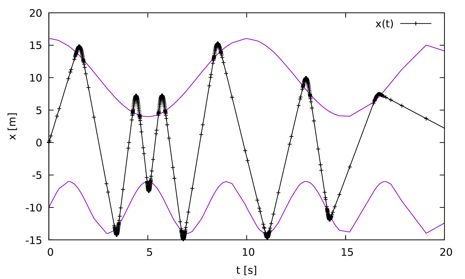
Fig. 3.11 The tennis players are moving. Note that the motion of the players is not well resolved, since the dynamic time stepping is not affected by their positions at all when the ball is in mid air. Also, the velocity of the ball is reduced when a player is moving backward during striking and enhanced when moving forward.
Warning
The usage of CustomMathExpression should be considered as last resort, since the call of a Python function is quite expensive compared to the execution of the generated C code. In particular, here one could have used heaviside((var("x")-self.top_position)/meter) to kick in the force of the racket instead. The division by meter is required in the argument of heaviside(), since functions like sin(), cos(), but also heaviside() require an argument without any dimension.