5.6.1. Damped Kuramoto-Sivashisky equation with periodic boundaries

Before delving into the stability analysis and bifurcation tracking, let us first define an interesting equation and integrate it temporally with pyoomph to see potential behavior of the equation. The example equation here will be the linearly and quadratically damped Kuramoto-Sivashinsky equation

(5.7)\[\begin{aligned} \partial_t h=-\gamma h-\delta h^2-\nabla^2 h -\nabla^4 h +\left(\nabla h\right)^2 \end{aligned}\]

This equation is already in its rescaled form with two nondimensional parameters \(\gamma\) and \(\delta\) controlling the damping. The field \(h\) can be interpreted as a height function. This equation has been proposed to reproduce pattern formation found in low-energy ion beam erosion of semiconductor surfaces, e.g. in Refs. [2, 15, 18].

When casting the equation to a weak form for pyoomph, we have to bear in mind that pyoomph does not allow for spatial derivatives beyond first order. Hence, we define \(g=\nabla^2h\) so that we obtain

\[\begin{split}\begin{aligned} \partial_t h&=-\gamma h-\delta h^2-\nabla^2 h -\nabla^2 g +\left(\nabla h\right)^2\\ g=&\nabla^2 h \end{aligned}\end{split}\]

and cast it into the weak formulation with test functions \(v\) and \(w\) for \(h\) and \(g\), respectively:

\[\begin{split}\begin{aligned} \left(\partial_t h+\gamma h+\delta h^2+\left(\nabla h\right)^2,v\right)+\left(g,w\right)&-\left(\nabla h+\nabla g,\nabla v\right)+\left(\nabla h,\nabla w\right)\\&+\left\langle \nabla h+\nabla g, \vec{n}v \right\rangle-\left\langle \nabla h, \vec{n}w \right\rangle=0 \end{aligned}\end{split}\]

Alternatively, of course, one could also add \(g\) to the first weak contribution term instead of the \(\nabla h\) term in the third contribution to account for the \(-\nabla^2h\) term in (5.7), which would yield different Neumann terms.

The implementation is straight-forward:

from pyoomph import *
from pyoomph.expressions import *
from pyoomph.expressions.utils import DeterministicRandomField  # for the random initial condition


class DampedKuramotoSivashinskyEquation(Equations):
    def __init__(self, gamma=0.0, delta=0.0, space="C2"):
        super(DampedKuramotoSivashinskyEquation, self).__init__()
        self.gamma, self.delta, self.space = gamma, delta, space

    def define_fields(self):
        self.define_scalar_field("h", "C2")  # h
        self.define_scalar_field("lapl_h", "C2")  # projection of div(grad(h))

    def define_residuals(self):
        h, v = var_and_test("h")
        lapl_h, w = var_and_test("lapl_h")
        self.add_residual(weak(partial_t(h) + self.gamma * h + self.delta * h ** 2 - dot(grad(h), grad(h)), v))
        self.add_residual(-weak(grad(h) + grad(lapl_h), grad(v)))
        self.add_residual(weak(lapl_h, w) + weak(grad(h), grad(w)))

For the problem, we want to use two new features, namely periodic boundaries and a random initial condition. We use a RectangularQuadMesh and connect the "left" with the "right" interface and the "top" with the "bottom" interface, so that the domain is virtually infinite in all directions due to periodicity. Thereby, there is no single Neumann term relevant. This can be done with the PeriodicBC, which must be added to an interface and gets the opposite interface as first argument. Furthermore, we must tell pyoomph, how to find the corresponding node on the other boundary to connect these. We can just pass an offset, so that each pair of nodes on both connected periodic boundary pair is found by applying this offset to the position of the source node to the destination node:

class KSEProblem(Problem):
    def __init__(self):
        super(KSEProblem, self).__init__()
        self.L = 50  # domain length
        self.N = 40  # number of elements
        self.gamma,self.delta=0.24,0.05 # parameters
        self.random_amplitude=0.01 # Initial random initial condition amplitude

    def define_problem(self):
        self.add_mesh(RectangularQuadMesh(N=self.N, size=self.L))

        eqs = DampedKuramotoSivashinskyEquation(gamma=self.gamma, delta=self.delta)
        eqs += MeshFileOutput()
        # Adding periodic boundaries: nodes at "bottom" will be merged by the nodes at top (found by applying offset to the position)
        eqs += PeriodicBC("top", offset=[0, self.L]) @ "bottom"
        # Same for the left<->right connection
        eqs += PeriodicBC("right", offset=[self.L, 0]) @ "left"

        # Create a deterministic random field. We must pass the corners of the domain
        # All random values will be pre-allocated so that successive evaluations of
        # the functions at the same point yield the same value
        h_init = DeterministicRandomField(min_x=[0, 0], max_x=[self.L, self.L], amplitude=self.random_amplitude)
        x, y = var(["coordinate_x", "coordinate_y"])
        eqs += InitialCondition(h=h_init(x, y))

        self.add_equations(eqs @ "domain")  # adding the equation

Warning

The PeriodicBC object enforces periodicity to all fields defined on this domain. It is hence not possible to have e.g. one field periodic and another one discontinuous across the interface with the PeriodicBC object.

Additionally, note that we use a DeterministicRandomField to create our initial condition. Since pyoomph requires that successive function calls with the same arguments yield the same values (i.e. deterministic functions), it is necessary to precalculate the random numbers in advance. This is done internally in the DeterministicRandomField. To that end, we must specify the minimum and maximum coordinates, so that internally an \(n\)-dimensional array of random numbers with the prescribed amplitude is created. Whenever the function is evaluated, it is interpolated between the initially generated random numbers to ensure the deterministic requirement.

The problem code is simple and representative results of the pattern formation are shown in Fig. 5.13:

if __name__ == "__main__":
    with KSEProblem() as problem:
        problem.run(2000, outstep=True, startstep=0.1, temporal_error=1, maxstep=50)

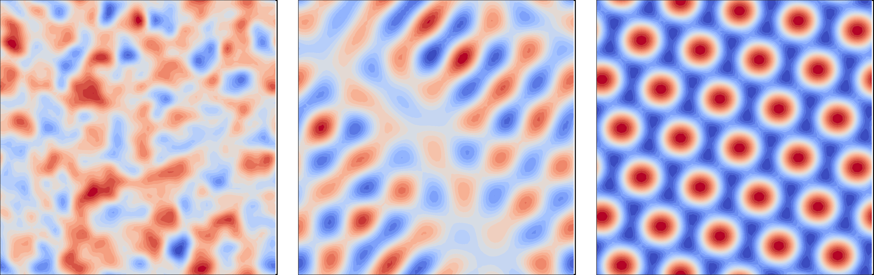
Fig. 5.13 Emergence of a hexagonal dot pattern by the damped Kuramoto-Sivashinsky equation starting from a random initial condition.

Download this example

Download all examples