5.6.2. Stability via eigenvalues
When simulating the damped Kuramoto-Sivashinsky for different values of \(\gamma\geq 0\) and \(\delta\geq 0\), one will notice that not only hexagonal dot patterns can emerge, but also hexagonal hole patters, stripe patters, but also even chaotic solutions can occur. Furthermore, when starting with a small amplitude of the random initial condition, just the simple solution \(h=0\) will be present if \(\gamma>1/4\). It is cumbersome to temporally integrate the equation for each combination of \(\gamma\) and \(\delta\) to create a phase diagram of the emerging solutions. Instead, one can use pyoomph’s features of eigenvalue calculation and bifurcation tracking to investigate the parameter space quickly.
To that end, we start with stationary solutions and test them for stability. However, we must have a good initial guess for the stationary solutions, since the stationary solve() command would not converge if we are too far off. In particular, it is helpful to know the typical length scale (or wave number \(k\)) of the emerging patterns. This can be done by linearizing (5.7) around \(h=0\) and investigate the spatially Fourier transformed equation:
Obviously, when \(\gamma>1/4\), the dispersion relation \(-\gamma+k^2-k^4\) is negative for all \(k=\|\vec{k}\|\). Therefore, all initial modes will decay over time. If \(\gamma\) is slightly below \(1/4\), the dispersion relation will have a positive maximum at the critical wave number \(k_\text{c}=k=1/\sqrt{2}\). Hence, we expect that the typical size of the emerging patterns, at least close to \(\gamma=1/4\), will be controlled by this wave number. Thereby, we can formulate several initial conditions, which will be used to find stationary solutions:
where the amplitude \(A\) can be used to control the amplitude of the initial conditions.
Of course, the domain size must be chosen that the initial conditions fit in perfectly. We therefore construct a new Problem class:
from kuramoto_sivanshinsky import * # Import the previous script

class KSEBifurcationProblem(Problem):
    def __init__(self):
        super(KSEBifurcationProblem, self).__init__()
        self.periods,self.period_y_factor=2,1 # consider two full periods in both directions
        self.N_per_period=20 # elements per period and direction
        self.kc=1/square_root(2) # wave number of the pattern
        # Introduce parameters
        # for both linear and quadratic damping with some initial settings
        self.param_gamma=self.define_global_parameter(gamma=0.24)
        self.param_delta=self.define_global_parameter(delta=0)


    def define_problem(self):
        kc, N = self.kc, self.N_per_period*self.periods
        Lx = self.periods * 4 * pi / kc # Calulate fitting mesh size
        Ly = self.period_y_factor*self.periods* 4 * square_root(1/3) * pi / kc
        mesh = RectangularQuadMesh(size=[Lx, Ly], N=[N, int(N* Ly / Lx)])
        self.add_mesh(mesh)

        eqs=MeshFileOutput()
        eqs+=DampedKuramotoSivashinskyEquation(gamma=self.param_gamma,delta=self.param_delta)

        # Register different initial conditions
        A=3
        x,y=var(["coordinate_x","coordinate_y"])
        eqs += InitialCondition(h=0,IC_name="flat")
        eqs += InitialCondition(h=2*A/9*(cos(kc*x)+2*cos(kc/2*x)*cos(kc*square_root(3)/2*y)),IC_name="hexdots")
        eqs += InitialCondition(h=-2 * A / 9 * (cos(kc * x) + 2 * cos(kc / 2 * x) * cos(kc * square_root(3) / 2 * y)),IC_name="hexholes")
        eqs += InitialCondition(h= A / 2 * cos(kc * x),IC_name="stripes")

        # And integral observables, in particular h_rms
        eqs += IntegralObservables(_area=1,_h_integral=var("h"),_h_sqr_integral=var("h")**2)
        eqs += IntegralObservables(h_avg=lambda _area,_h_integral : _h_integral/_area)
        eqs += IntegralObservables(h_rms=lambda _area, h_avg,_h_sqr_integral: square_root(_h_sqr_integral/_area - h_avg**2))
The parameters \(\gamma\) and \(\delta\) are now bound as parameters, i.e. we can change the values dynamically during the simulation. Moreover, we pass IC_name arguments to the InitialCondition objects. Thereby, we can later on set the different starting conditions by set_initial_condition(). The four initial conditions are plotted in Fig. 5.14.
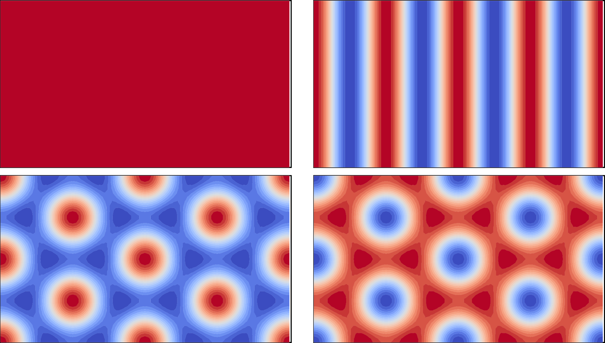
Fig. 5.14 Initial conditions used as initial guesses for the stationary solutions.
One might wonder why we do not add PeriodicBC boundaries here. The reason is that we later on want to calculate stationary solutions and eigenvalues. Since (5.7) is invariant with respect to a shift of the coordinate system, any stationary solution \(h_0\) would automatically imply an infinite set of stationary solutions \(h_{0,\vec{s}}(\vec{x})=h_0(\vec{x}-\vec{\text{s}})\). And each of these solutions would have eigenvalues of zero corresponding to this shift, i.e. with eigenfunctions \(\nabla h_0\cdot{s}\). This would hamper the stability analysis tremendously. Instead, we fix the arbitrary shift (and the rotational freedom due to the isotropy of (5.7)) by omitting the PeriodicBC. Thereby, zero Neumann fluxes will be imposed a the boundaries, i.e. \(\partial_x h=\partial_x^3 h=0\) at the "left" and "right" boundaries and \(\partial_y h=\partial_y^3 h=0\) at the "top" and "bottom" boundaries will be present.
Furthermore, we add IntegralObservables here. These are observables of the type
i.e. we integrate the argument over the "domain" here. Thereby, we can calculate the "_area" of the "domain" by integrating over 1. Furthermore, we integrate over \(h\) and store it in "_h_integral". The underscore just indicates that its output should be suppressed, since both the "_area" and the "_h_integral" are just helper observables we require to determine the root mean square of the field. The root mean square (rms) is given by
Obviously, the terms cannot be written in a form like (5.8), but we can use lambda calls to evaluate mathematical expressions based on integral observables. \(h_\text{avg}\) is obviously just the quotient of "_h_integral" and "_area", so we bind it via the lambda as such. For the rms, we first write it as equivalent
and bind this observable via a lambda.
First, let us investigate only the case \(\delta=0\) for varying \(\gamma\):
# slepc eigensolver is more reliable here
import pyoomph.solvers.petsc # Requires petsc4py, slepc4py. Might not work in Windows

if __name__ == "__main__":
    with KSEBifurcationProblem() as problem:
        problem.initialise()
        problem.param_gamma.value=0.24
        problem.param_delta.value = 0.0
        problem.set_initial_condition(ic_name="hexdots") # set the hexdot initial condition
        problem.solve(timestep=10) # One transient step to converge towards the stationary solution
        problem.solve() # stationary solve

        problem.set_eigensolver("slepc") # Set the slepc eigensolver
        # Write eigenvalues to file
        eigenfile=open(os.path.join(problem.get_output_directory(),"hexdots.txt"),"w")
        def output_with_eigen():
            eigvals,eigvects=problem.solve_eigenproblem(6,shift=0) # solve for 6 eigenvalues with zero shift
            h_rms=problem.get_mesh("domain").evaluate_observable("h_rms") # get the root mean square
            line=[problem.param_gamma.value,h_rms,eigvals[0].real,eigvals[0].imag] # line to write
            eigenfile.write("\t".join(map(str,line))+"\n") # write to file
            eigenfile.flush()
            problem.output_at_increased_time() # and write the output

        # Arclength continuation
        output_with_eigen()
                  while problem.param_gamma.value>0.23:
                      ds=problem.arclength_continuation(problem.param_gamma,ds,max_ds=0.005)
                      output_with_eigen()
We use another eigensolver, provided by the PETSc/SLEPc package. These can be installed as explained in Section 2.4.
These packages might not be available in Windows. Just give it a try. If these packages cannot be installed, you can omit the import and the set_eigensolver() call to use the default scipy eigensolver.
We then jump on the stationary solution by a stationary solve() command. However, before we step a bit in the direction with a transient solve command, since we might otherwise converge into the flat solution \(h=0\). We perform an arclength_continuation() along \(\gamma\) and output the eigenvalue with the largest real part and the calculated rms to a text file. Based on the real part of the eigenvalue, we can determine whether the stationary solution is stable or not. The results are depicted in Fig. 5.15, where we also include the flat solution, which stability has been investigate analytically before.
The rms is used as y-axis to show the amplitude of the patterns. Obviously, for \(\delta=0\), hexagonal dot structures cease to exist for \(\gamma\geq 0.2826\) in a fold bifurcation. Between \(\gamma=0.25\) and this value, both the flat solution and hexagonal dot solutions co-exists with a hysteretic behavior in this range.
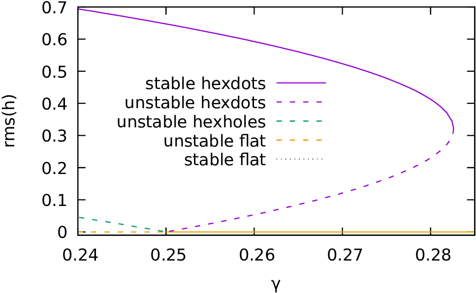
Fig. 5.15 Fold bifurcation at \(\gamma\approx 0.2826\), where hexagonal dots stops to exist. For higher \(\gamma\), only the flat solution exists. Below \(\gamma<0.25\), hexagonal dot structures are the generic solution, at least in the shown interval. The hexagonal hole branch is unstable and meets the flat solution in a transcritical bifurcation.