5.6.3. Stability via bifurcation tracking
We could now perform similar scans for different \(\delta\), but there is a simpler route, namely bifurcation tracking. We can instruct pyoomph to find the fold bifurcation and its corresponding value of \(\gamma\approx 0.2826\) directly:
from kuramoto_sivanshinsky_arclength_eigen import * # Import the previous example problem

if __name__ == "__main__":
    with KSEBifurcationProblem() as problem:
        # Output the zeroth eigenvector. Will only output if the eigenvalue/vector is calculated either by
        # solve_eigenproblem or by bifurcation tracking
        problem.additional_equations+=MeshFileOutput(eigenvector=0,eigenmode="real",filetrunk="eigen0_real")@"domain"

        problem.initialise()
        problem.param_gamma.value=0.24
        problem.param_delta.value = 0.0
        problem.set_initial_condition(ic_name="hexdots")
        problem.solve(timestep=10) # One transient step to converge towards the stationary solution
        problem.solve() # stationary solve

        # from the previous example we know that the fold bifurcation happens close to 0.28
        problem.param_gamma.value=0.28
        problem.solve() # solve at gamma=0.28

        # Activate bifurcation tracking
        problem.activate_bifurcation_tracking(problem.param_gamma,"fold")
        problem.solve()
        print("FOLD BIFURCATION HAPPENS AT",problem.param_gamma.value)
To that end, we first move close to the bifurcation, i.e. to \(\gamma=0.28\) and solve() to find a good guess. Then, we activate_bifurcation_tracking() for a "fold" bifurcation in \(\gamma\). Within the next solve() command, the value of \(\gamma\) will be adjusted (i.e. \(\gamma\) is in fact a degree of freedom) so that the system is directly at the fold bifurcation. We also output the eigenvector directly at the fold bifurcation. To that end, another MeshFileOutput is added, but with the arguments eigenvector=0 (meaning the zeroth eigenvector) and eigenmode="real" (i.e. considering the real part, although this particular eigenvector is real anyhow). We furthermore must supply a filetrunk to prevent overwriting of the output files of the solution itself.
Once we are on the bifurcation, we can sweep over \(\delta\) and follow the position of the fold bifurcation. As long as the bifurcation tracking is active \(\gamma\) will be adjusted to stay on the fold bifurcation, i.e. we get a curve \(\gamma_\text{fold}(\delta)\), which is written to file:
        hexfold_file = open(os.path.join(problem.get_output_directory(), "hexfold.txt"), "w")
        def output_with_params():
            h_rms = problem.get_mesh("domain").evaluate_observable("h_rms")  # get the root mean square
            line = [problem.param_gamma.value, problem.param_delta.value,h_rms]  # line to write
            hexfold_file.write("\t".join(map(str, line)) + "\n")  # write to file
            hexfold_file.flush()
            problem.output_at_increased_time()  # and write the output

        output_with_params()
        ds = 0.025
        while problem.param_delta.value < 0.5:
            ds = problem.arclength_continuation(problem.param_delta, ds, max_ds=0.025)
            output_with_params()
The result, i.e. the location of the fold bifurcation, is depicted in Fig. 5.16.
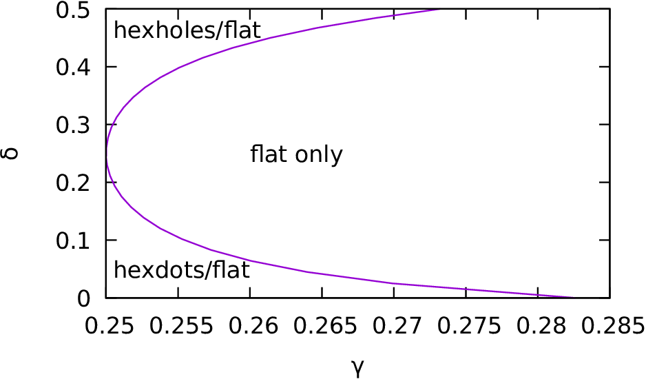
Fig. 5.16 Emergence of a hexagonal dot pattern by the damped Kuramoto-Sivashinsky equation starting from a random initial condition.
Similarly, we can set the other InitialCondition to start with hexagonal holes or stripe patterns and find the bifurcations.