5.3.2. Transient and nonlinear generalization of Stokes’ law
Please refer to Section 4.4.7 for understanding the problem setup. We will only address the required changes here.
First of all, we do not only have to balance the drag force \(F_\text{d}\) with the buoyancy force \(F_g\), but also the inertia \(M\dot{U}\) matters, where \(M\) is the mass of the spherical object. To that end, instead of using the GlobalLagrangeMultiplier we write a simple ODEEquations class to account for Newton’s law of motion:
class NewtonEquation(ODEEquations):
    def __init__(self,M,F_buo):
        super(NewtonEquation, self).__init__()
        self.M, self.F_buo = M, F_buo

    def define_fields(self):
        self.define_ode_variable("UStokes",scale="velocity",testscale=1/scale_factor("force"))

    def define_residuals(self):
        U,V=var_and_test("UStokes")
        self.add_residual(weak(self.M*partial_t(U)-self.F_buo,V))
As in the previous example, to this equation of motion, the drag force will be added externally by the DragContribution added to the interface of fluid and object.
In the problem class, to minimize errors stemming from the imposition of the pure Stokes solution at the far field, we shrink the spherical object and increase the radius of the far field:
        self.sphere_radius = 0.25 * milli * meter  # radius of the spherical object
        self.outer_radius = 50 * milli * meter  # radius of the far boundary
Since we have a temporal problem, also a time scale has to be set
self.set_scaling(temporal=self.sphere_radius/UStokes_ana)
We then have to exchange the StokesEquations by the NavierStokesEquations to account for the inertia. However, when transforming into the co-moving frame of reference, we have to correct for the acceleration of the co-moving system. This can be added via the bulkforce argument, which adds a contribution proportional to \(\rho_\text{l}\dot{U}\vec{e}_z\) to the NavierStokesEquations. This effectively changes the time derivative in the inertia to \(\rho_\text{l}(\partial_t \vec{u}-\dot{U} \vec{e}_z)\) so that the acceleration of the coordinate system \(\dot{U}\) cancels out:
        U = var("UStokes", domain="globals")  # bind U from the domain "globals"
        inertia_correction=self.fluid_density*vector([0,1])*partial_t(U)
        eqs = NavierStokesEquations(dynamic_viscosity=self.fluid_viscosity,mass_density=self.fluid_density,bulkforce=inertia_correction)  # Stokes equation and output
Instead of the GlobalLagrangeMultiplier we add the developed NewtonEquation:
        # Define the Lagrange multiplier U
        U_eqs=NewtonEquation(4/3*pi*self.sphere_radius**3*self.sphere_density,F_buo)
        U_eqs+=ODEFileOutput()
        self.add_equations(U_eqs @ "globals")  # add it to an ODE domain named "globals"
Note that we combine it with an ODEFileOutput to write the time evolution of \(U(t)\) to a file.
Finally, the run code must be transient now:
if __name__ == "__main__":
    with TransientNonlinearStokesLawProblem() as problem:
        problem.run(0.5*second,startstep=0.05*second,outstep=True)  # solve and output
As seen in Fig. 5.7, the final velocity field is not symmetric anymore and a transient dynamics of \(U(t)\) is plotted.
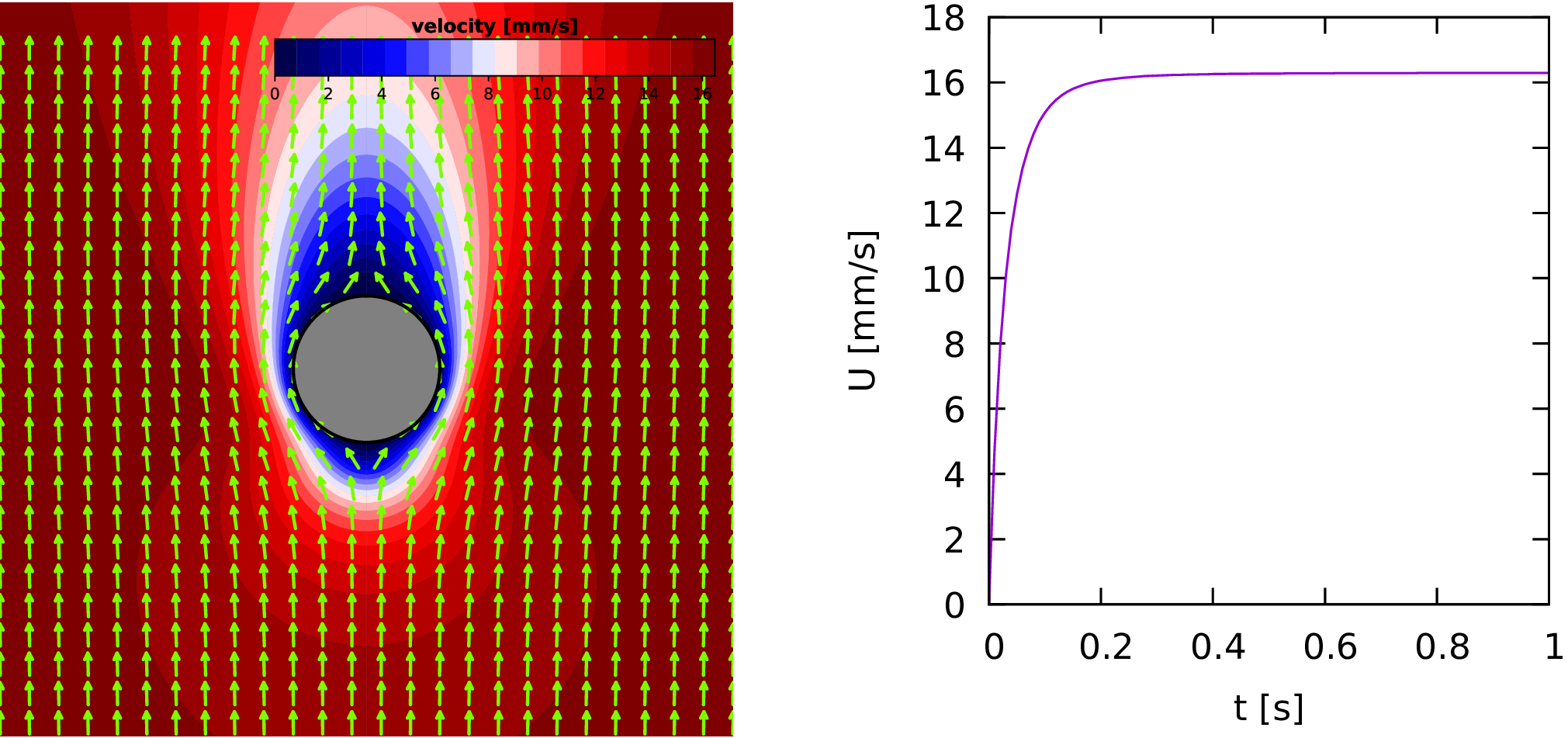
Fig. 5.7 (left) Velocity around a spherical object with consideration of inertia. (right) Evolution of the velocity \(U(t)\).