5.3.4. Marangoni instability
Another interesting instability that can arise in a system that combines the Navier-Stokes equation (velocity \(\vec{u}\), pressure \(p\)) with an advection-diffusion equation (scalar field \(c\)) is the Marangoni instability. This instability is driven by a combination of the non-linear advection term \(\vec{u}\cdot\nabla c\) and a surface tension \(\sigma=\sigma(c)\) that depends on \(c\). Obviously, we must impose a surface tension force, in particular a tangential traction due to potential surface tension gradient along the interface. As in the previous example, we use the predefined classes NavierStokesEquations and AdvectionDiffusionEquations, where the velocity of the former is used to advect the field \(c\) in the latter. The field \(c\) just couples back via a tangential traction at the top interface. We will additionally use physical dimensions for this example:
from pyoomph import *
# Use the pre-defined equations for Navier-Stokes and advection-diffusion
from pyoomph.equations.navier_stokes import *
from pyoomph.equations.advection_diffusion import *

# Dimensional problem
from pyoomph.expressions.units import *

class MarangoniProblem(Problem):
	def __init__(self):
		super(MarangoniProblem,self).__init__()
		self.W,self.H=1*milli*meter, 0.25*milli*meter # Size of the box
		self.rho,self.mu=1000*kilogram/meter**3, 1*milli*pascal*second  # density and viscosity
		self.D=1e-9*meter**2/second # diffusivity
		self.Nx=10 # elmenents in x-direction
		self.max_refinement_level=3 # max. 4 times refining
		self.dsigma_dc=-0.1*milli*newton/meter

	def define_problem(self):
		self.set_scaling(spatial=self.W,temporal=0.1*second)
		self.set_scaling(velocity=scale_factor("spatial")/scale_factor("temporal"))
		self.set_scaling(pressure=1*pascal)
		# add the mesh
		self.add_mesh(RectangularQuadMesh(size=[self.W,self.H],N=[self.Nx,int(self.Nx*self.H/self.W)]))
		eqs=MeshFileOutput() # output

		eqs+=AdvectionDiffusionEquations(fieldnames="c",wind=var("velocity"),diffusivity=self.D,space="C1")
		eqs+=NavierStokesEquations(dynamic_viscosity=self.mu,mass_density=self.rho)
		# Initial condition
		xrel,yrel=var("coordinate_x")/self.W,var("coordinate_y")/self.H
		eqs+=InitialCondition(c=yrel*(1+0.01*cos(2*pi*xrel)+0.001*sin(4*pi*xrel)))
		# Refinements based on c and velocity
		eqs+=SpatialErrorEstimator(c=1,velocity=1)
		# Adding no-slip conditions
		for wall in ["left","right","bottom"]:
			eqs+=DirichletBC(velocity_x=0,velocity_y=0)@wall

		# "Free" surface: fixed y-velocity, Marangoni force
		sigma=self.dsigma_dc*var("c")		# Surface tension
		eqs+=(DirichletBC(velocity_y=0)+NeumannBC(velocity=-grad(sigma)))@"top"
		# Fix one pressure degree
		eqs+=DirichletBC(pressure=0)@"bottom/left"
		self.add_equations(eqs@"domain")


if __name__=="__main__":
	with MarangoniProblem() as problem:
		# problem.dsigma_dc=0.1*milli*newton/meter
		problem.run(1*second,outstep=True,startstep=0.01*second,maxstep=0.1*second,spatial_adapt=1,temporal_error=1)
Since we have a dimensional problem now, all quantities as e.g. rho and mu and also the size of the box W\(\times\)H are dimensional. To nondimensionalize, we have to set the spatial and temporal scales, as well as the pressure and velocity scale. The scale of the field c is not set, since we use a non-dimensional field for \(c\). Thereby, the problem gets nondimensionalized internally. As initial condition for \(c\), we have a linear gradient in \(y\) direction (lower \(c\) in the bulk as compared to the "top" interface) with a tiny tangential perturbation. The "left", "right" and "bottom" sides are just no-slip boundary conditions.
At the "top" interface, we just set the \(y\)-velocity to zero, i.e. the liquid is not allowed to flow out of the domain. Furthermore, we define the surface tension \(\sigma=c\,\partial_c \sigma\), i.e. linearly dependent on the field \(c\). The factor dsigma_dc controls the direction, i.e. whether the surface tension increases or decreases with \(c\). The absolute value of the surface tension does not matter in this setting, since we only calculate tangential gradients thereof. To apply the Marangoni force, we just add a NeumannBC that applies the traction. The minus sign stems from the fact, that the Neumann term \(\langle \cdot,\cdot\rangle\) in (4.13) is negative. Since the gradient of the surface tension will only have contributions in \(x\)-direction, it is indeed just a tangential contribution, i.e. applied on the \(x\)-direction of the velocity. In total, this means that we apply the tangential Marangoni traction \(t_x=\partial_x \sigma\).
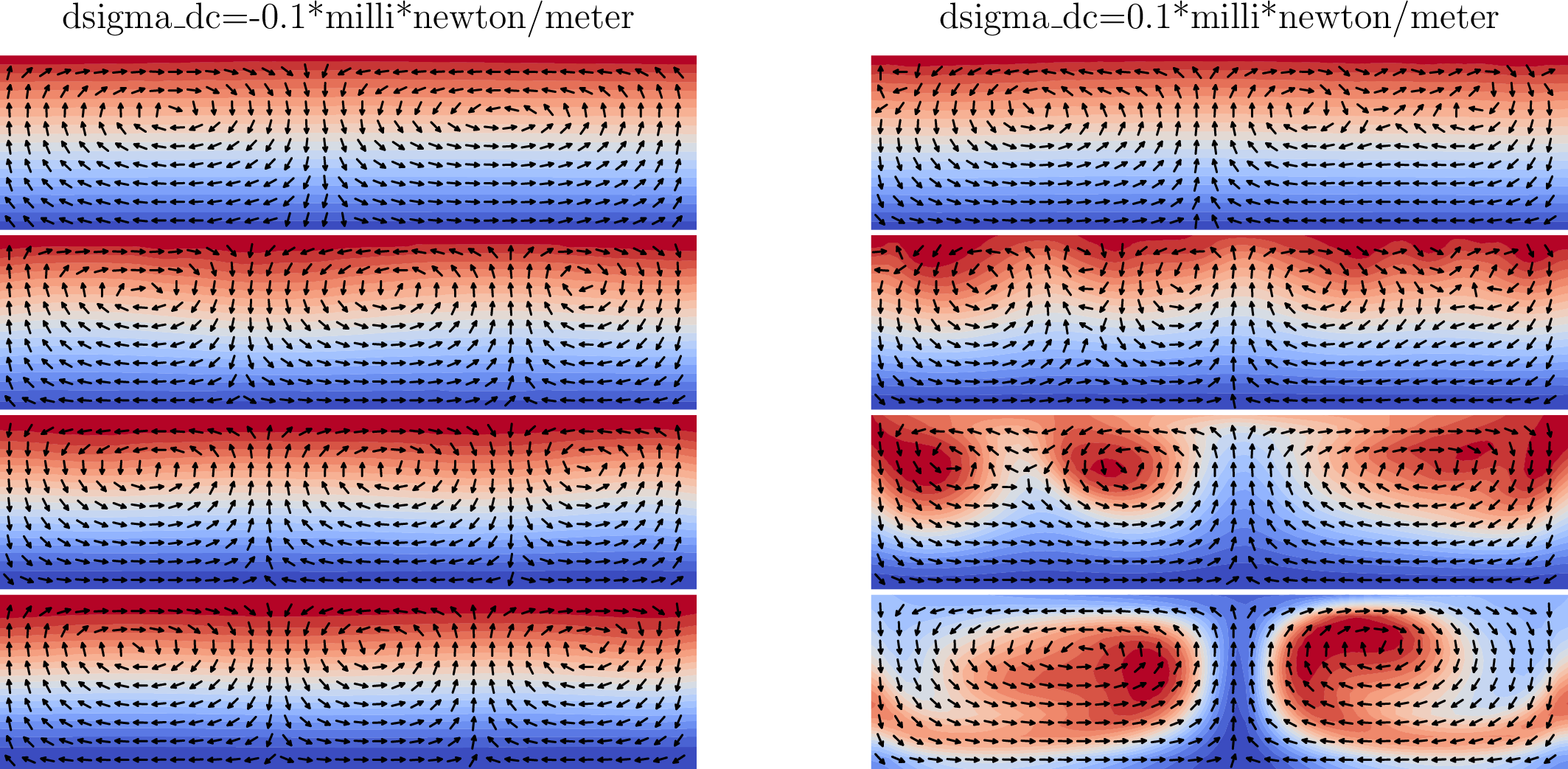
Fig. 5.9 Marangoni (in)stability. (left) When the surface tension decreases with \(c\), i.e. \(\partial_c \sigma<0\), the surface is stable. (right) when \(\sigma\) increases with \(c\), we have initially a higher surface tension than the liquid in the bulk would yield. Any tiny perturbation can pull up liquid from the bulk, locally reducing the surface tension even more and enhancing the perturbation. This can easily result in chaotic dynamics.
As apparent from Fig. 5.9, we see a drastic effect of whether \(\partial_c \sigma\) is positive or negative. When \(\partial_c \sigma\) is negative, any perturbation at the interface will be damped out. Any Marangoni flow will pull up liquids with higher surface tension to the positions with previously lower surface tension. Thereby, the Marangoni flow gets hampered over time. If, however, \(\partial_c \sigma>0\), it is vice versa: Any perturbation will pull up liquid with lower surface tension to spots where already a lower surface tension was before. Thereby, the Marangoni instability is triggered, leading to a self-enhancing Marangoni effect that eventually breaks up into chaotic flow. Of course, if the gradient of \(c\) in bulk direction would be inverted, i.e. higher \(c\) in the bulk as compared to the interface, also the dynamics would be unstable for \(\partial_c\sigma<0\) and stable for \(\partial_c\sigma>0\).
It is remarkable that the tiny perturbation and the tiny dependence \(\partial_c \sigma\) of the surface tension on the field \(c\) are sufficient to trigger this chaotic dynamics. However, the Marangoni number, i.e. the nondimensional number to estimate the Marangoni effect, has the viscosity and in particular the diffusivity in the denominator. Both these quantities are so small that the Marangoni number is in fact large.
The Marangoni instability is the explanation why e.g. evaporating droplets consisting of ethanol and water are chaotic, whereas evaporating droplets consisting of glycerol and water show regular flow.