8.5. Example: Marangoni instability in a Hele-Shaw cell
We want to investigate the Marangoni instability (cf. Section 5.3.4) of an evaporating ethanol-water mixture which is confined between two plates at the top and bottom, i.e. by a Hele-Shaw cell. The flow in such a cell is usually three-dimensional, but when the plate distance \(\delta\) is small compared to the flow structures, one can assume that the flow in \(z\)-direction (i.e. the direction between both plates) is parabolic due to the no-slip boundary conditions at the top and bottom plate, i.e. at \(z=0\) and \(z=\delta\). The velocity \(\vec{u}_\text{3d}(x,y,z,t)\) is then just given by the average flow \(\vec{u}(x,y,t)\) by \(\vec{u}_\text{3d}=6z(\delta-z)\vec{u}/\delta^2\). The presence of the no-slip boundary conditions modify the Navier-Stokes equations for the projected two-dimensional by a factor \(6/5\) for the nonlinear term and an additional Brinkman term of \(-12\mu\vec{u}/\delta^2\):
In pyoomph, we can just pass the plate distance \(\delta\) via the hele_shaw_thickness argument to the CompositionFlowEquations() to automatically account for these modifications of the Navier-Stokes equations.
Experimentally, numerically and analytically, this setting has been investigated in Ref. [10]. Here, we will use the multi-component equations of pyoomph to reprocude the problem by simulation:
from pyoomph import *
from pyoomph.equations.multi_component import *
from pyoomph.expressions.utils import * # for the random perturbation
from pyoomph.materials import *
import pyoomph.materials.default_materials # Alternatively, define the materials by hand


class MarangoniHeleShawProblem(Problem):
    def __init__(self):
        super(MarangoniHeleShawProblem, self).__init__()
        # domain size: Gas size is the same as domain_length
        self.domain_length,self.domain_width=0.5*milli*meter,0.5*milli*meter
        self.cell_thickness=20*micro*meter # Hele-Shaw plate distance
        self.Nx=18 # Num elements in x direction
        self.max_refinement_level=3 # max refinement level to refine near the interface
        self.temperature=20*celsius # Temperature : Required for some properties
        self.liquid_mixture = Mixture(get_pure_liquid("water") + 0.5 * get_pure_liquid("ethanol"))  # Default liquid mixture
        # The gas mixture must be adjusted: In the experiment, the evaporation happens in 3d space
        # Here, it is just two-dimensional so the Green's function of the Poisson equation for diffusion is not bounded!
        # Therefore, we pin the vapor concentration at the far right to this composition
        self.gas_mixture = Mixture(get_pure_gas("air") + 20*percent * get_pure_gas("ethanol") + 40*percent * get_pure_gas("water"),quantity="relative_humidity",temperature=self.temperature)
        self.interface_props=None # Interface properties, are determined automatically if not set
In the experiments, the evaporation happens in open space. Here, we only have a two-dimensional setting. While in 3d the ambient conditions could be imposed at infinite distances due to the far field decay of \(1/r\) with the distance \(r\) of the vapor concentration from the interface, in 2d it does not work: The corresponding Green’s function is \(\ln(r)\) and hence it is not bounded at infinity. Therefore, we must strongly impose the vapor concentration at a finite distance. This artificial vapor concentration can be set with by the composition of the gas_mixture and must be adjusted so that the typical evaporation rates match with the experiment.
Again, in the define_problem(), we setup the spatial and temporal scale by hand and let the remaining scales be determined automatically from the properties of the liquid_mixture. However, we adjust the velocity and pressure scale by hand afterwards to better match the typical orders of magnitude for this particular problem (e.g. by measurements in the experiments). Since properties may depend on the temperature and potentially the absolute_pressure, we must again set these on a global (i.e. Problem-wide) level with the define_named_var():
def define_problem(self):
    # Spatial and temporal scales must be set by hand
    self.set_scaling(spatial=self.domain_length, temporal=1 * second)
    # Set remaining scales by the liquid properties
    self.liquid_mixture.set_reference_scaling_to_problem(self, temperature=self.temperature)
    # Adjust pressure and velocity a bit to the problem
    self.set_scaling(pressure=10 * pascal, velocity=1e-4 * meter / second)
    # define global constants "temperature" and "absolute_pressure". It might be required by the fluid properties
    self.define_named_var(temperature=self.temperature, absolute_pressure=1 * atm)
The mesh is just a RectangularQuadMesh, but it has to be separated into two domains. This is possible if we pass a function to the argument name. Pyoomph will evaluate this function in the center of each element (in non-dimensional coordinates, i.e. measured in the spatial scale) and add these elements to the domain by this name. Here, we mark all elements that are on the left half as "liquid", whereas the elements on the right half are in the "gas" domain. If an internal facet is between two elements of different domains, it will be automatically added to the interface named by the two domains (in alphabetical order) separated by an underscore, i.e. here the liquid-gas interface will be automatically named "gas_liquid":
# Mesh: All elements with center further away than 1*domain_length (measured in spatial scale) will be gas, otherwise liquid
domain_func=lambda x,y: "gas" if x>1 else "liquid"
mesh=RectangularQuadMesh(size=[2*self.domain_length,self.domain_width],N=[2*self.Nx,int(self.Nx*self.domain_width/self.domain_length)],name=domain_func)
self.add_mesh(mesh)
Then, the equations have to be assembled. If the user does not explicitly selects the interface_props by hand, it will be determined from the material library:
# We can either set the interface properties by hand, e.g. to modify the surface tension
# if not, we must find it from the material library
if self.interface_props is None:
    # To get the interface properties, we can just use the | operator
    self.interface_props=self.liquid_mixture | self.gas_mixture
    # When a particular liquid-gas interface is not defined, it will use a default interface
    # This one will use a reasonable mass transfer model and the default_surface_tension["gas"] of the liquid properties

liq_eqs=MeshFileOutput()
# Flow with Hele-Shaw confinement and use second order for the composition
liq_eqs+=CompositionFlowEquations(self.liquid_mixture,hele_shaw_thickness=self.cell_thickness,compo_space="C2",spatial_errors=True)
liq_eqs+=DirichletBC(velocity_y=0)@"bottom"
liq_eqs += DirichletBC(velocity_y=0) @ "top"
liq_eqs+=MultiComponentNavierStokesInterface(self.interface_props)@"gas_liquid"
liq_eqs+=RefineToLevel()@"gas_liquid" # And refine it to max_refinement_level
The liquid equations mainly consist of the CompositionFlowEquations() with the liquid_mixture properties and the given hele_shaw_thickness along with a few boundary conditions and a static MultiComponentNavierStokesInterface with the interface_props. As discussed in the section before, the latter will automatically impose a free surface (static here, since no equations for mesh motion are added) with the surface_tension property of the interface_props. Also the evaporation model is considered and it will couple automatically to the "gas" domain. Note that we switch the space of the advection-diffusion equations for the required mass fraction fields to "C2", i.e. second order fields and also add spatial_errors for the spatial adaptivity. The free interface is always refined to the maximum level by the RefineToLevel object.
The gas equations are now just CompositionDiffusionEquations() with a prescribed far field DirichletBC based on the initial composition of the gas_mixture:
# Gas
gas_eqs=MeshFileOutput()
gas_eqs+=CompositionDiffusionEquations(self.gas_mixture) # just diffusion
# And fix the far boundary to the initial condition by iterating over all advection diffusion fields for the mass fractions
gas_eqs+=DirichletBC(**{"massfrac_"+c:True for c in self.gas_mixture.required_adv_diff_fields})@"right"

self.add_equations(liq_eqs@"liquid"+gas_eqs@"gas")
To run the simulation, we first slightly perturb the initial condition directly at the interface with random numbers. Thereby, the instability kicks in earlier, whereas otherwise, due to perfect symmetry of the mesh, it would start rather late just by the accumulation of tiny numerical errors of the Newton solver:
if __name__=="__main__":
    with MarangoniHeleShawProblem() as problem:
        # Slightly perturb the interface
        # 10 random numbers with a small amplitude linearily interpolated on the interval 0:1
        randpert=DeterministicRandomField(min_x=[0],max_x=[1],amplitude=0.002,Nresolution=10)
        yn=var("coordinate_y")/problem.domain_width # normalized coordinate
        randpert=randpert(yn) # interpolated random fields
        # Perturb the interface composition slightly
        problem.additional_equations+=InitialCondition(massfrac_ethanol=problem.liquid_mixture.initial_condition["massfrac_ethanol"]+randpert)@"liquid/gas_liquid"
        problem.run(10*second,startstep=0.01*second,maxstep=0.5*second,outstep=True,temporal_error=1,spatial_adapt=1)
The results are depicted in Fig. 8.2 and indeed show the experimentally observed coarsening and merging arch-like patterns. For a smaller plate distance, the growing of the arches can be suppressed due to the stronger damping of the Brinkman term in (8.5), whereas without the hele_shaw_thickness argument (e.g. by setting problem.cell_thickness=None) for the CompositionFlowEquations() (i.e. just the normal 2d Navier-Stokes), a violent chaotic flow would emerge.
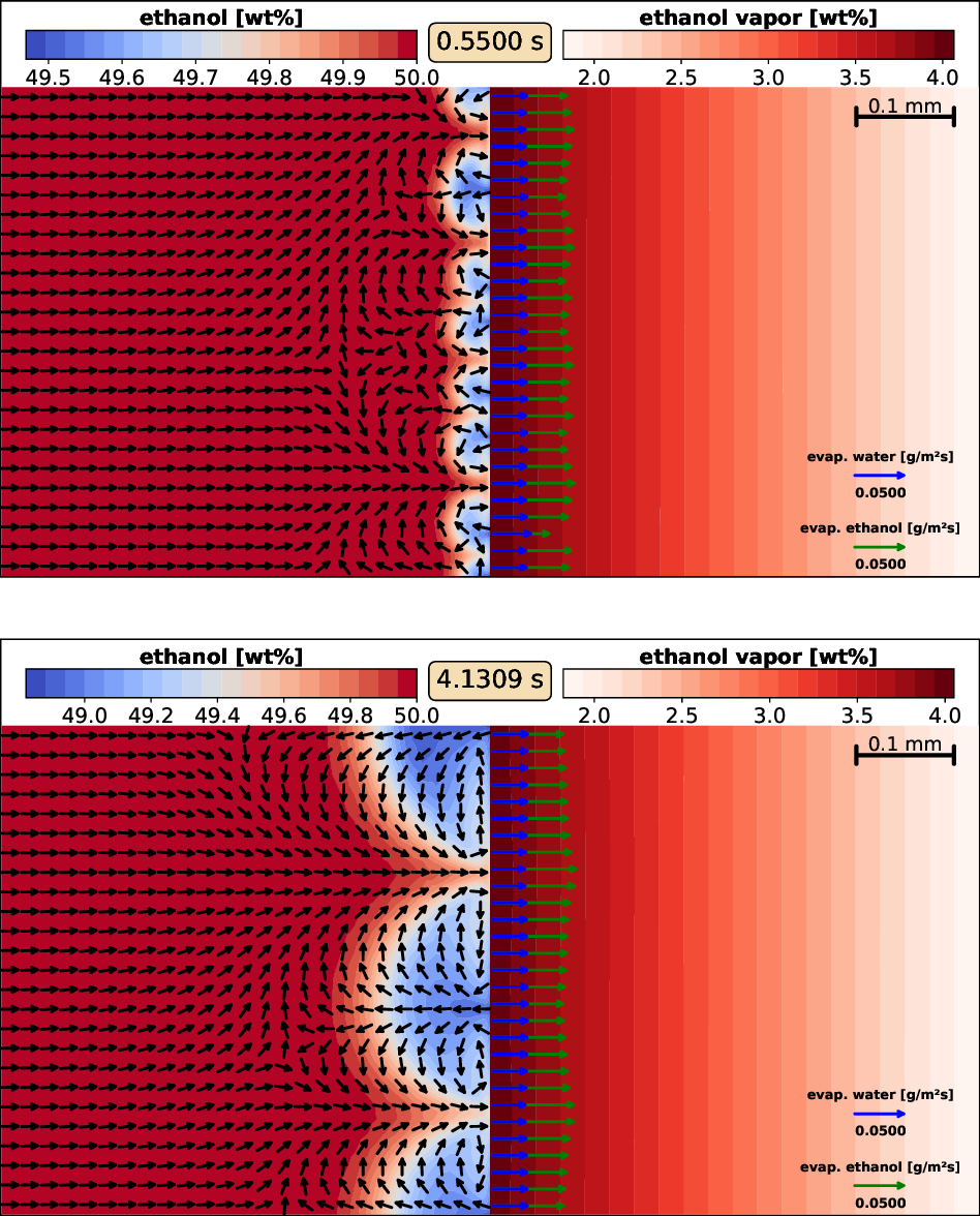
Fig. 8.2 Marangoni instability of an ethanol-water mixture evaporating in a Hele-Shaw cell.