8.3. Example: Rayleigh-Taylor instability
Similar to the problem discussed in Section 5.3.3, we now want to set up the same problem with the CompositionFlowEquations():
from pyoomph import *
from pyoomph.equations.multi_component import *
from pyoomph.materials import *
import pyoomph.materials.default_materials # Alternatively, define the materials by hand

class RayleighTaylorProblem(Problem):
    def __init__(self):
        super(RayleighTaylorProblem, self).__init__()
        self.box_height,self.box_width=1*milli*meter,0.25*milli*meter # box size
        self.Nx=5 # Num elements in x direction
        self.mixture=Mixture(get_pure_liquid("water")+0.5*get_pure_liquid("glycerol")) # Default mixture
        self.temperature=20*celsius # Temperature : Required for some properties
        self.gravity=9.81*vector(0,-1)*meter/second**2
We import the material library and also the default materials. Alternatively, we could write our own material library file or define custom fluids and mixtures thereof in the very same python script of the code. Then, we initialize the property Mixture() by a default mixture, but in the run script, the user can change it easily.
For the define_problem() method, we first have to set the spatial and the temporal scale. All other required scales can be set to reasonable values by using the set_reference_scaling_to_problem() of the liquid:
    def define_problem(self):
        # Mesh
        self.add_mesh(RectangularQuadMesh(size=[self.box_width,self.box_height],N=[self.Nx,int(self.Nx*self.box_height/self.box_width)]))
        # Spatial and temporal scales must be set by hand
        self.set_scaling(spatial=self.box_width,temporal=1*second)
        # Set remaining scales by the liquid properties
        self.mixture.set_reference_scaling_to_problem(self,temperature=self.temperature)
        # define global constants "temperature" and "absolute_pressure". It might be required by the fluid properties
        self.define_named_var(temperature=self.temperature,absolute_pressure=1*atm)
It is important to pass the temperature variable here since set_reference_scaling_to_problem() internally evaluates e.g. the dynamic_viscosity and mass_density to find a good scaling. Since these properties might depend on the temperature, we must supply some temperature for that. Furthermore, the initial composition is substituted in these expressions so that eventually only constant values appear for the reference density and viscosity used for the non-dimensionalization.
Furthermore, since the problem is isothermal and also pressure fluctuations are not allowed to have an effect on the fluid properties, we must tell pyoomph what to use for the fields "temperature" and "absolute_pressure", when any fluid property depends on these. Therefore, we set these variables globally to constants by the define_named_var(). Whenever pyoomph finds any occurrence of e.g. var("temperature") and there is no such field defined in the current domain, these values will be used instead. Thereby, all temperature-dependence will just be evaluated at this constant value. Since this substitution and successive simplification of the properties happens before the C code generation, a potential temperature-dependence of the fluid properties does not slow down the simulation.
The code is now just a CompositionFlowEquations() of the Mixture() with the desired gravity:
        eqs=MeshFileOutput()
        eqs+=CompositionFlowEquations(self.mixture,spatial_errors=True,gravity=self.gravity)
        for side in ["left","right","bottom"]:
            eqs+=DirichletBC(velocity_x=0,velocity_y=True)@side
            # Top side must be open: The density is not constant and hence we require in/outflow somewhere!

        self.add_equations(eqs@"domain")
For the boundary conditions, however, we have to be careful: Since the mass density is in general not constant, the total volume will not be conserved. Hence, one side of the domain must allow for in-/outflow. Alternatively, we could also apply a no-slip condition at the "top" interface, but pass the argument boussinesq=True to the CompositionFlowEquations(). In that case, the Boussinesq approximation is applied, i.e. the continuity equation simplifies to \(\nabla\cdot \vec{u}=0\). Then, the volume remains conserved, but we have to fix one degree of the pressure again (cf. Section 4.4.4).
Finally, the user can change the Mixture() and prescribe any suitable InitialCondition for the liquid:
with RayleighTaylorProblem() as problem:
    # Let the user select any mixture
    problem.mixture = Mixture(get_pure_liquid("water") + 0.5 * get_pure_liquid("glycerol"))

    # And also formulate the initial condition
    x,y=var(["coordinate_x","coordinate_y"])
    xrel, yrel = var("coordinate_x") / problem.box_width, var("coordinate_y") / problem.box_height - 0.5
    wg_init = 0.5*(1+tanh(100 * (yrel - 0.0125 * cos(2 * pi * xrel))))
    problem.additional_equations+=InitialCondition(massfrac_glycerol=wg_init)@"domain"

    problem.max_refinement_level=4
    problem.run(10*second,startstep=0.1*second,maxstep=0.5*second,outstep=True,spatial_adapt=1,temporal_error=1)
The results are shown in Fig. 8.1. Due to the high viscosity and low diffusivity in the limit of pure glycerol, the flow and diffusion dynamics mostly happen in the lower half.
The benefit of using the material library is that it is now trivial to exchange it for e.g. an ethanol-water mixture or even ternary mixtures with just a single line of code (provided the desired fluids and mixtures thereof are already in the material library).
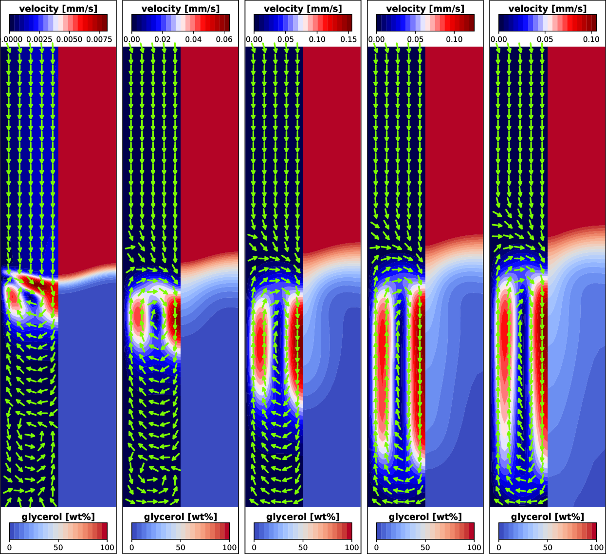
Fig. 8.1 Rayleigh-Taylor instability in the glycerol-water system.