9.1. Advection-diffusion equation with an upwind scheme
To illustrate how to define the necessary facet terms in the weak formulation of DG methods, we will refer back to the example of the advection-diffusion equation from Section 5.2.2 where we discussed the SUPG stabilization.
In strong formulation, we want to solve
Upon multiplication with a test function \(d\) and subsequent spatial integration, we get
Our first focus is now the advection term, \((\nabla \cdot (\vec{u} c),d)\), which can be split into the contributions of each element \(E\), i.e.
Here, \(\vec{n}\) is the normal pointing outward at each point on the boundary \(\partial E\) of each element \(E\). Opposed to continuous Galerkin methods, \(\vec{u}\) and \(c\) may be different on both sides of the boundary in discontinuous Galerkin methods. This means that the integrations along the interior element boundaries \(\partial E\) do not cancel out by the corresponding interior boundary contribution of the adjacent element.
Nevertheless, the boundary integrals can be rearranged into the contributions of each facet \(F\), shared by two elements \(E^+\) and \(E^-\). Each facet is only defined once in the mesh, even if it is shared by two elements. The facet normal \(\vec{n}\) is pointing from the element \(E^+\) to the element \(E^-\). The particular order, i.e. which element is assigned as \(E^+\) and \(E^-\) viewed from each facet \(F\) is irrelevant here. We can now write it as bulk integration over the full domain \(\Omega\), its exterior boundary \(\partial \Omega\), and the interior facets \(F\):
Note that \(\vec{n}^-=-\vec{n}^+\) holds, since the nodal coordinates are always continuous in pyoomph (however, it might not hold on curved manifold with a co-dimension). Also, we assume a continuous given velocity field, so that \(\vec{u}^-=-\vec{u}^+\) holds as well. In CG methods, also \(c^-=c^+\) and \(d^-=d^+\) holds, so that the facet terms indeed cancel out. In DG methods, however, this is not the case. In fact, the interaction of \(c^+\) and \(c^-\) across the facet must be explicitly implemented in a reasonable way that reflects the nature of the equation. Here, we have to make sure that whatever is transported from one element to the other is also removed from the first element. To that end, we apply here the upwind scheme by transporting \(c^+\) if \(\vec{n}^+\cdot\vec{u}^+>0\) and \(c^-\) otherwise. To that end, we define an auxiliary velocity normal to the facet, which makes sure to account only for upwind transport and vanishes otherwise
and rewrite the facet terms of the advection by
Obviously, either \(u_n^{\text{up},+}\) or \(u_n^{\text{up},-}\) is positive and the other one vanishes. Thereby, we either transport \(c^+\) or \(c^-\), depending on the direction of the velocity, by removing this flux from one element and adding it to the other, i.e. ensure conservation.
Since such jump terms, i.e. the difference of an expression on the two sides of a facet, are common in DG methods, pyoomph offers the function jump(), which lets you write the above expression in pyoomph in a shorter notation. This will be addressed later in the implementation.
For the diffusion term, similar facet terms must be derived. Doing the same splitting in bulk contribution, exterior boundary, and interior facets, we get
where we abbreviated the diffusive fluxes through the facet by
Opposed to the upwind scheme for advection, the diffusive fluxes should be considered in a symmetric way, i.e. we can define the average on both sides
For such a term, we can use the avg() function in pyoomph, which calculates the average of the expression on both sides of the facet. This will be addressed later in the implementation as well. Similar to the transport by advection, the diffusive fluxes must be removed from one element and added to the other, i.e. we must ensure conservation, which can be done by replacing the facet terms stemming from diffusion by
While this considers a conservative and reasonable diffusive transport across the facet, this form neither penalizes huge jumps in the concentration \(c\) (which should be smoothed by diffusion) nor is it symmetric. For a symmetric, consistent and coercive formulation we can weakly enforce continuity of \(c\) in the sense of Nitsche’s method by adding a symmetric and a penalty term to the facet terms, i.e. we write
Here, \(\alpha\) is a penalty parameter and \(h\) is the average element size of both elements attached to the facet. The penalty term ensures coercivity of the problem, i.e. the existence of a unique solution. The penalty parameter \(\alpha\) should be chosen large enough to ensure coercivity, but small enough to not dominate the solution. The average element size \(h\) is calculated by the average of the element sizes of both elements attached to the facet.
For the implementation, the equation starts as usual. We can pass an arbitrary finite element space, continuous or discontinuous:
class ConvectionDiffusionEquation(Equations):
    def __init__(self, u, D ,space="C2",alpha_DG=2):
        super(ConvectionDiffusionEquation, self).__init__()
        self.u = u  # advection velocity
        self.D = D  # diffusivity
        self.space=space
        # Activate interior facet terms if the space is discontinuous
        self.requires_interior_facet_terms=is_DG_space(self.space)
        self.alpha_DG=alpha_DG # penalty parameter for DG

    def define_fields(self):
        self.define_scalar_field("c", self.space)
Whenever facet terms must be added, as here, we must set the property requires_interior_facet_terms to True. This will trigger the generation of an interior skeleton mesh which includes all interior facets of the mesh. Exterior boundaries are not part of this skeleton mesh. Each facet appears only once in the interior skeleton mesh, although each interior facet is shared by two elements.
As an auxiliary method, the function is_DG_space() is used, which automatically detects if the space is discontinuous.
The definition of the weak form now also tests whether we have an continuous space or must add additional facet terms:
    def define_residuals(self):
        c, ctest = var_and_test("c")
        # Conventional form, used for CG spaces
        self.add_weak(partial_t(c), ctest)
        self.add_weak(self.D * grad(c) -self.u*c, grad(ctest))

        if is_DG_space(self.space):
            # Additional facet terms for DG spaces
            h_avg=avg(var("cartesian_element_length_h")) # length of an element:
            n=var("normal") # in facet terms, the normal vector is the facet normal. For the element normal, var("normal",domain="..") can be used.
            # if used without any restriction, i.e. outside from jump or average, it will default to n^+

            # Upwind scheme. See whether the velocity is in the direction of the normal vector, otherwise, it will be zero
            un_upwind=(dot(self.u, n) + absolute(dot(self.u, n)))/2

            # Assemble the facet terms:
            facet_terms=weak(self.D*(self.alpha_DG/h_avg)*jump(c),jump(ctest))
            facet_terms=-weak(self.D*jump(c)*n,avg(grad(ctest)))
            facet_terms=-weak(self.D*avg(grad(c)),jump(ctest)*n)
            facet_terms+=weak( jump(un_upwind*c,at_facet=True) ,jump(ctest))

            # And add them to the skeleton mesh of the facets
            self.add_interior_facet_residual(facet_terms)
Again, we make use of is_DG_space() to check whether the space is discontinuous. If this is the case, we define the facet terms.
For these terms, we first define the upwind convection, which is only giving a contribution if the velocity is advecting in the same direction as the facet normal, which can be bound by var("normal"). The normal of the element itself, i.e. not the facet normal, can be obtained by var("normal",domain=".."). This is a consequence from the expansions of the variables at the domain where you add the residual terms, which are here the facets. For the elements, you hence must go one level up in the domain hierarchy.
We furthermore define the average element length \(h\), which is calculated by the average avg() of both element sizes attached to the facet. The element size can be obtained by the special variable name var("cartesian_element_length_h"). You can also use var("element_length_h") instead, which is identical for Cartesian coordinate systems, however, for other coordinate systems, both will differ. In fact, these lengths are calculated by integrating the elemental length/area/volume (depending on the element dimension \(N_\text{el}\)) and subsequently taking the \(N_\text{el}\)-th root of the result. The length/area/volume calculation is done in a Cartesian coordinate system for var("cartesian_element_length_h") and in the coordinate system of the current equations for var("element_length_h"). In dimensional problems, both consider the scaling scale_factor("spatial"), i.e. \(h\) will be measured in meters if the problem is dimensional.
Also, we use jump() to calculate the jumps of the variables across the facets. By default, both avg() and jump() expands all contained variables at the bulk element domains on both sides. Both attached bulk elements can also be accessed directly via the domains "+" and "-". Here, we could e.g. replace avg(var("cartesian_element_length_h")) by (var("cartesian_element_length_h",domain="+"))+var("cartesian_element_length_h",domain="-"))/2, which is exactly what avg() does.
However, in the last jump(), we want to calculate the jump of the upwind convection term. Since this term requires the facet normal, we must make sure that var("normal") is indeed evaluated at both sides of the facet, not the attached bulk elements. Therefore, we must use the at_facet=True flag to indicate that the variables should be expanded at the facet domain. It is also possible to explicitly expand on both sides of the facet domain by using the domains "+|" and "|-", respectively.
Note that one cannot know a priori which element is on the "+" and which is on the "-" side of the facet. The order of the elements is not guaranteed. However, in reasonable formulations of such facet terms, the order of the elements should not matter.
Finally, we add the facet terms to the skeleton mesh of the facets by the add_interior_facet_residual() method.
The problem code reads as before, but we use the keyword argument discontinuous=True to obtain a better output to include the discontinuities. Thereby, each element writes its nodes individually to the output, i.e. overlapping nodes are multiple times present in the output. The same also works for the MeshFileOutput class to write VTU files in higher dimensions. The default discontinuous=False will just take the average value at overlapping nodes for the output.
class OneDimAdvectionDiffusionProblem(Problem):
    def __init__(self):
        super(OneDimAdvectionDiffusionProblem, self).__init__()
        self.u=vector(1,0)
        self.D=0.0001
        self.space="D1"

    def define_problem(self):
        self.add_mesh(LineMesh(N=100,size=100,minimum=-20)) # coarse mesh from [-20:80]

        eqs=TextFileOutput(discontinuous=True)
        eqs+=ConvectionDiffusionEquation(u=self.u,D=self.D,space=self.space)

        x=var("coordinate_x")
        cinit=exp(-x**2*0.25)
        eqs+=InitialCondition(c=cinit)

        self.add_equations(eqs@"domain")


if __name__=="__main__":
    with OneDimAdvectionDiffusionProblem() as problem:
        problem.run(50,outstep=1,maxstep=0.1)
The discontinuous output is plotted in Fig. 9.1.
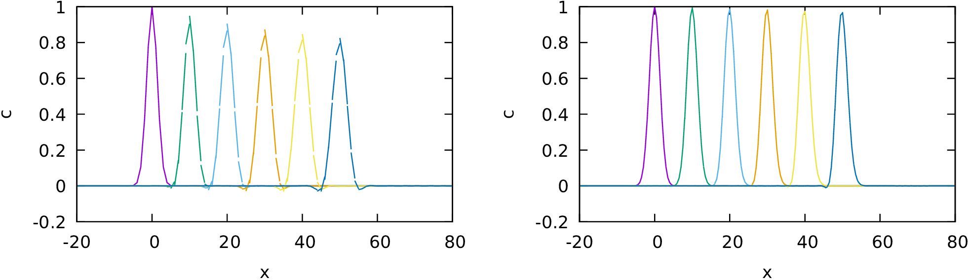
Fig. 9.1 Discontinuous Galerkin method for the advection-diffusion equation on spaces "D1" (left) and "D2" (right). The solution is shown at time steps of 10. The discontinuities are clearly visible. Also, "D1" has too few degrees of freedom, which leads to severe numerical diffusion. This is typical for underresolved upwind schemes, as also seen in the SUPG implementation, cf. Fig. 5.5.
Note
It is easily possible to switch the upwind scheme by a central scheme by replacing un_upwind by
un_central=dot(self.u, n)/2