5.2.2. SUPG implementation
An analogous approach to the upwind scheme in finite differences is the SUPG stabilization in the finite element method. In the upwind scheme, the first order advective derivative is evaluated in the upwind direction, i.e. taking the slope in the upwind direction, which stabilizes the scheme for high Péclet numbers. The SUPG method (streamline upwind Petrov-Galerkin) does essentially the same in the finite element method. However, while it is trivial to find the degrees of freedom in the upwind direction on a regular line or 2d/3d grid in the finite difference method, for arbitrary meshes, as commonly used in the finite element method, it is not that trivial.
The one-dimensional problem is best to illustrate the idea, so we will stick to it here. The general idea is to weight the upwind residuals more, i.e. to modify the localization of the residual by the projection on the test function to be enhanced in upwind direction. This can be achieved by replacing the test function \(\phi\) in (5.3) by \(\phi+\tau\vec{u}\cdot\nabla \phi\). The choice of the parameter \(\tau\) is crucial and will be discussed in a minute. The SUPG variant of (5.3) (with \(\nabla\cdot \vec{u}=0\) and for pure Dirichlet boundary conditions) hence reads (cf. e.g. [3]):
We have assumed a first order space ("C1") here (or vanishing diffusivity \(D\)), which removes the term \(D\nabla^2c\) in the last weak contribution. Pyoomph cannot handle second order derivatives yet, so this approximation is also necessary at the moment for "C2" spaces, where \(\nabla^2c\) does not vanish in each element. The selection of \(\tau\) is important. There are several approaches, but usually it is defined as a constant per element. It must have a finite value for \(\vec{u}\to 0\), and must compensate the \(\vec{u}\) term in the test function argument of the last term of (5.5) to prevent a dominance of the stabilization term for high velocities. Furthermore, it must vanish for infinitely refined meshes (so it must depend on the element size). The idea is to introduce the mesh Péclet number
where \(h\) is the size of the current element (e.g. the length of a one-dimensional element or the circumference for 2d elements). When \(\operatorname{Pe}_h\to 0\), we do not require any stabilization, which happens for low velocities, high diffusivities or small elements. If \(\operatorname{Pe}_h\) becomes large (typically \(>3\)), stabilization is necessary to prevent the spurious oscillations for advection-dominated problems. Hence, a good selection of \(\tau\) is
The term in the brackets indeed is \(0\) for \(\operatorname{Pe}_h=0\) and goes to unity for large \(\operatorname{Pe}_h\). The factor \(\frac{h}{\|\vec{u}\|}\) compensates for the \(\nabla\) and the velocity appearing in the stabilization projection on \(\tau\vec{u}\cdot\nabla\phi\).
To augment the advection-diffusion equations with the stabilization term, we can use the class ElementSizeForSUPG from pyoomph.equations.SUPG. It will calculate the Cartesian measure (i.e. length/area/volume) of each element and store it in a "D0" space. Since in moving mesh methods (cf. Section 6) the elements can change in size, the element size becomes part of the degrees of freedom. One can access the typical element length scale by the method get_element_h() of the ElementSizeForSUPG object.
The implementation of the augmented form (5.5) reads:
from pyoomph import *
from pyoomph.equations.SUPG import * # To calculate the element size


class ConvectionDiffusionEquationWithSUPG(Equations):
    def __init__(self, u, D,with_SUPG=True):
        super(ConvectionDiffusionEquationWithSUPG, self).__init__()
        self.u = u  # advection velocity
        self.D = D  # diffusivity
        self.scheme="TPZ" # Time scheme, trapezoidal rule
        self.with_SUPG=with_SUPG # do we activate SUPG?

    def define_fields(self):
        self.define_scalar_field("c", "C1") # Take the coarse space C1

    def get_supg_tau(self):
        # We must find an equation of the type ElementSizeForSUPG, which calculates the element size
        elsize_eqs = self.get_combined_equations().get_equation_of_type(ElementSizeForSUPG, always_as_list=True)
        if len(elsize_eqs)!=1: # User must combine it with a single ElementSizeForSUPG instance
            raise RuntimeError("SUPG only works if combined with a single ElementSizeForSUPG equation")
        elsize_eqs=elsize_eqs[0] # get the ElementSizeForSUPG object, which is combined with this equation
        h = elsize_eqs.get_element_h() + 1e-15 # element size, add a tiny offset to prevent errors
        u_mag=square_root(dot(self.u,self.u))+1e-15 # velocity magnitude , add a tiny offset to prevent errors
        Pe_h=u_mag*h/(2*self.D) # Mesh Peclet number
        beta=1/tanh(Pe_h)-1/Pe_h # coefficient activating SUPG if Pe becomes large
        tau = subexpression(beta*h/(2*u_mag)) # returning the tau coefficient
        return tau

    def define_residuals(self):
        c, ctest = var_and_test("c")
        # This term occurs multiple times, so wrap it into a subexpression for performance gain
        radv = subexpression(time_scheme(self.scheme,partial_t(c) + dot(self.u, grad(c))))
        self.add_residual(weak(radv, ctest))  # time derivative and advection
        self.add_residual(time_scheme(self.scheme,weak(self.D * grad(c), grad(ctest))))  # diffusion
        if self.with_SUPG: # SUPG stabilization
            self.add_residual(time_scheme(self.scheme,weak(radv,self.get_supg_tau() * dot(self.u, grad(ctest)))))
In the method get_supg_tau we check if the equation is combined with a single ElementSizeForSUPG object and bind the size \(h\). We calculate \(\operatorname{Pe}_h\) and thereby \(\tau_h\) according to the relations discussed above. Finally, this is used for the stabilization term, but only if with_SUPG is True.
As a test class, we advect again a bump, but this time in one dimension:
class OneDimAdvectionDiffusionProblem(Problem):
    def __init__(self):
        super(OneDimAdvectionDiffusionProblem, self).__init__()
        self.u=vector(1,0)
        self.D=0.0001
        self.with_SUPG=True

    def define_problem(self):
        self.add_mesh(LineMesh(N=100,size=100,minimum=-20)) # coarse mesh from [-20:80]

        eqs=TextFileOutput()
        eqs+=ConvectionDiffusionEquationWithSUPG(u=self.u,D=self.D,with_SUPG=self.with_SUPG)
        if self.with_SUPG:
            eqs+=ElementSizeForSUPG() # We must add the element size

        x=var("coordinate_x")
        cinit=exp(-x**2*0.25)
        eqs+=InitialCondition(c=cinit)

        eqs+=DirichletBC(c=0)@"left"
        eqs += DirichletBC(c=0) @ "right"

        self.add_equations(eqs@"domain")
It is necessary to add an ElementSizeForSUPG object to calculate the element size if SUPG is active. The rest is trivial, but note that we again use DirichletBC on both sides. Neumann conditions would have to be augmented by SUPG correction terms stemming from the consistent partial integration that leads to (5.5).
With a simple run code, we can compare the results with and without SUPG:
if __name__=="__main__":
    with OneDimAdvectionDiffusionProblem() as problem:
        problem.with_SUPG=True
        problem.run(50,outstep=1,maxstep=0.1)
Results are depicted in Fig. 5.5.
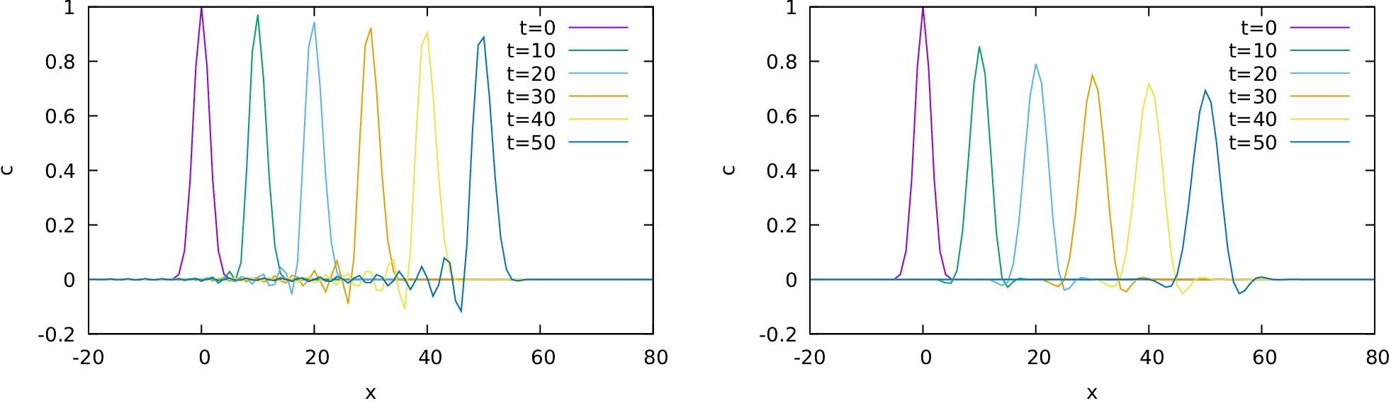
Fig. 5.5 Without (left) and with SUPG (right). Note how spurious oscillations are suppressed by SUPG, but the bump diffuses too fast. When the number of elements is increased, both problems vanish, even without SUPG.
Note
An alternative way of getting the typical element size is just using var("cartesian_element_size_Eulerian") or var("element_size_Eulerian") instead of ElementSizeForSUPG. See var() for more information on such keyword variables.