9.2. Weakly imposing Dirichlet boundary conditions
The last example illustrated how the continuity of the concentration field \(c\) across the facets can be enforced in a weak sense by adding facet terms. If you use the conventional DirichletBC on the exterior boundaries, it will enforce the conditions strongly, also in discontinuous Galerkin methods. However, in some cases, you may want to enforce the Dirichlet boundary conditions weakly, i.e. in the same way as the facet terms. In order to easily switch between continuous and discontinuous Galerkin spaces, one can still use the DirichletBC class, but one has to add the implementation of the weak Dirichlet boundary conditions manually to the equation class. This will be discussed in the following.
We consider a simple Poisson equation, again implemented for both continuous and discontinuous Galerkin spaces. The facet terms can be directly copied from the diffusion term of the advection-diffusion equation. The only modification we do is adding the keyword argument allow_DL_and_D0=True to the test for discontinuous spaces via the is_DG_space() function. Thereby, we can use the discontinous spaces without degrees of freedom at the nodes, i.e. "DL" and "D0", as well.
class PoissonEquations(Equations):
             def __init__(self,f,space,alpha_DG=4):
                 super().__init__()
                 self.f=f
                 self.space=space
                 self.requires_interior_facet_terms=is_DG_space(self.space, allow_DL_and_D0=True)
                 self.alpha_DG=alpha_DG

             def define_fields(self):
                  self.define_scalar_field("u",self.space)

             def define_residuals(self):
                 u,v=var_and_test("u")
                 # Both continuous and discontinuous spaces
                 self.add_residual(weak(grad(u),grad(v))-weak(self.f,v))
                 if is_DG_space(self.space, allow_DL_and_D0=True):
                   # Discontinuous penalization
                   h_avg=avg(var("cartesian_element_length_h"))
                   n=var("normal") # will default to n^+ if used without any restriction in facets

                   facet_terms= weak(self.alpha_DG/h_avg*jump(u),jump(v))
                   facet_terms-=weak(jump(u)*n,avg(grad(v)))
                   facet_terms-=weak(avg(grad(u)),jump(v)*n)
                   self.add_interior_facet_residual(facet_terms)
However, we now also add a special function which gives the correct weak terms for weakly imposed Dirichlet boundary conditions. This function must return the weak terms that are necessary to enforce some particular Dirichlet value. These are essentially the same as the facet terms, however, instead of jump(), we just take the current value on the boundary minus the prescribed value. The function avg() is just replaced by the evaluation of the variable on the boundary. In case we do not provide such a field or the field is continuous, we just return None, advising the DirichletBC to impose the value strongy:
def get_weak_dirichlet_terms_for_DG(self, fieldname, value):
   if fieldname!="u" or not is_DG_space(self.space, allow_DL_and_D0=True):
      return None
   else:
      u,v=var_and_test("u",domain="..") # bind the bulk field to get bulk gradients
      n=var("normal") # exterior normal
      h=var("cartesian_element_length_h",domain="..") # element size of the bulk element
      facet_terms=weak(self.alpha_DG/h*(u-value),v)
      facet_terms-=weak((u-value)*n,grad(v))
      facet_terms-=weak(grad(u),v*n)
      return facet_terms
The problem is as usual, but we allow to select the space and whether we want to use the weak Dirichlet boundary conditions when possible:
class PoissonProblem(Problem):
   def __init__(self):
      super().__init__()
      x=var("coordinate")
      self.f=500.0*exp(-((x[0] - 0.5)** 2 + (x[1] )**2)/ 0.02)
      self.space="D1"
      self.prefer_weak_dirichlet=True
      self.alpha_DG=4
      self.N=8

   def define_problem(self):
      self+=RectangularQuadMesh(N=self.N)
      eqs=MeshFileOutput(discontinuous=True)
      eqs+=PoissonEquations(self.f,self.space,self.alpha_DG)
      eqs+=DirichletBC(u=0,prefer_weak_for_DG=self.prefer_weak_dirichlet)@["left","right","top","bottom"]
      self+=eqs@"domain"

with PoissonProblem() as problem:
   problem.solve()
   problem.output()
By default, DirichletBC will impose the conditions weakly whenever the equations in the bulk provide corresponding facet terms by the method get_weak_dirichlet_terms_for_DG(). If this function returns None or if the keyword argument prefer_weak_for_DG in DirichletBC is set to False, the conditions will be imposed strongly. The output is shown in Fig. 9.2.
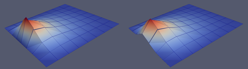
Fig. 9.2 Strongly (left) and weakly (right) imposed Dirichlet boundary conditions. While the strongly imposed conditions exactly fulfill the relation at the boundaries, they induce stronger discontinuities in the bulk. Upon refinement, both approaches converge to the same correct solution.
Finally, we want to address that the discontinous Galerkin implementation can easily be switched to a finite volume method. In such methods, quantities are usually element-wise constant, i.e. approximated on the space "D0". If setting space="D0", all terms involving grad(u) and grad(v) will vanish, since the gradients are zero in the element-wise constant space. The weak formulation will hence only read
i.e. we only integate over the source \(f\) in the bulk and the fluxes are just represented by the jumps of the field values. The flux terms can be understood as finite difference approximation of the fluxes, i.e. we just take the difference of the values at the cell centers, divided by the distance \(h_\text{avg}\). While \(\alpha\) is a penalty parameter for higher order polynominal approximations, it is now crucial to set the penalty parameter to \(\alpha=1\) to recover the correct finite difference approximations when using the "D0" space. Upon setting space="D0" and alpha_DG=1 and increasing the number of elements to N=40, we obtain the solution plotted on the left side of Fig. 9.3.
Discontinous Galerkin methods can hence be understood as generalization of finite volume methods by allowing for higher order polynominal approximations inside the elements. However, it is important to note that if we use e.g. a second order space, "D2", as depicted on the right side of Fig. 9.3, it is necessary to increase the penalty parameter (here we used \(\alpha=6\)) to obtain stable solution.
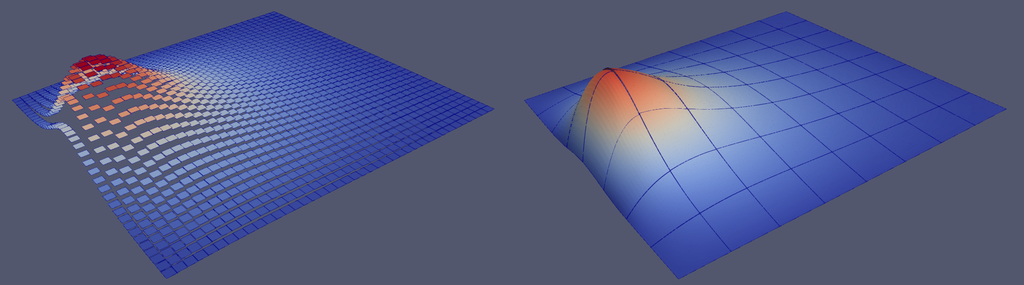
Fig. 9.3 (left) Using the space "D0" requires to set \(\alpha=1\) and resembles a finite volume method. (right) for the "D2" space it is necessary to increase the penalty parameter.