6.8.2. Compression of 2D circular disk
Note
The following case is a direct adaption of the corresponding example in oomph-lib.
We consider a 2d disc that is compressed by a uniform pressure. The disc initially has a radius of unity, however, we introduce an isotropic growth factor of \(\Gamma=1.1\), so that the disc wants to grow to a radius of \(\sqrt{\Gamma}\) in absence of any external pressure. Opposed to the corresponding example in oomph-lib, we will come up with two implementations of the very same case. We either can solve the problem on a quarter circle mesh with symmetry boundary conditions in a two-dimensional Cartesian coordinate system. However, due to the coordinate-system agnostic formulation of equations, the same can be realized by a simple radial line mesh in a polar coordinate system. To that end, we introduce a flag polar_implementation in the problem class:
from pyoomph import *
from pyoomph.expressions import *
from pyoomph.equations.solid import *
from pyoomph.meshes.simplemeshes import CircularMesh

class CompressedDiscProblem(Problem):
    def __init__(self):
        super().__init__()
        self.Gamma=1.1 # isotropic growth factor
        self.P=self.define_global_parameter(P=0) # Pressure on the circumference of the disc
        self.polar_implementation=True # Use radial polar coordinates only
         # Generalized Hookean solid constitutive law
        self.claw=GeneralizedHookeanSolidConstitutiveLaw(E=1,nu=0.3)

    def define_problem(self):
        # Base equations, irrespective of the coordinate system
        eqs=MeshFileOutput()
        eqs+=DeformableSolidEquations(constitutive_law=self.claw,coordinate_space="C2",isotropic_growth_factor=self.Gamma)
        eqs+=SolidNormalTraction(self.P)@"circumference"

        # Mesh, coordinate system and boundary conditions depending on whether we solve a 2d Cartesian or polar 1d problem
        if self.polar_implementation:
            self+=LineMesh(size=1,N=20,left_name="center",right_name="circumference") # Create a line mesh for the radial direction
            self.set_coordinate_system("axisymmetric") # Polar coordinate system
            eqs+=DirichletBC(mesh_x=0)@"center" # Fixed in the center of the disc
        else:
            # Case of Cartesian coordinates, we create a quarter circular mesh
            self+=CircularMesh(radius=1,segments=["NE"])
            eqs+=DirichletBC(mesh_x=0)@"center_to_north" # and fix the positions at the symmetry axes
            eqs+=DirichletBC(mesh_y=0)@"center_to_east"
The basis setup is analogous to the previous example, i.e. we require a constitutive law which is then used in the DeformableSolidEquations. Here, however, we impose the isotropic_growth_factor, which lets the disc grow everywhere from its undeformed configuration by \(\Gamma\) in terms of the area. Again, a SolidNormalTraction is imposed at the boundary circumference. If polar_implementation==True, we switch to an axisymmetric` coordinate system (which is a radial polar coordinate system for 1d meshes) and use a simple 1d mesh. In that case, the right boundary will be called circumference, whereas the left boundary of the interval is called center. At the latter, we make sure that the mesh position is fixed to the origin. If we do not solve the polar case, we do solve it on a quarter circle mesh on a 2d Cartesian coordinate system. We have to fix the mesh coordinates on the axes of symmetry in that case.
We also want to measure the current radius \(r\) of the disc. Irrespective of the coordinate system, we can do so by integrating over the boundary circumference. We calculate two integrals, namely the line length \(L=\int 1\:\mathrm{d}l\) and the integral over the radius \(R=\int \|\vec{x}\|\:\mathrm{d}l\). In case of the 2d Cartesian implementation, both integrals will be only a quarter of the full disc, but this does not matter, since the (averaged) radius of the disc can be obtained by the ratio \(r=R/L\):
        # To monitor the radius of the disc, we can use IntegralObservables. We integrate over the circumference of the disc to the the line length
        # and we also integrate over r*dl
        eqs+=IntegralObservables(_linelength=1,_radius_integral=square_root(dot(var("coordinate"),var("coordinate"))))@"circumference"
        # The radius is then given by the ratio of the integral of r and the line length
        eqs+=IntegralObservables(radius=lambda _radius_integral,_linelength:_radius_integral/_linelength)@"circumference"

        self+=eqs@"domain"
In the driver code, we just iterate over the imposed pressure (starting with a negative pressure to pull the disc outwards first). To compare the actual radius \(r\) with an analytical linearized expression (see the oomph-lib example for details), we can evaluate the introduced observable and write both the numerical value and the analytical approximation to a text file in the output directory:
with CompressedDiscProblem() as problem:
    delta_p=0.0125
    nstep=21

    problem.P.value=-delta_p*(nstep-1)*0.5 # Start with a negative pressure (pulling the disc outwards)
    problem.initialise()
    problem.refine_uniformly()

    # Write a comparison output file with the radius computed from the linearized analytical solution and the numerical solution
    outf=problem.create_text_file_output("disc_output.txt",header=["P","r_numeric","r_linear"])

    for i in range(nstep):
        problem.solve()
        problem.output_at_increased_time()
        rlinear=square_root(problem.Gamma)*(1-problem.P*(1+problem.claw.nu)*(1-2*problem.claw.nu))
        rnumeric=problem.get_mesh("domain/circumference").evaluate_observable("radius")
        outf.add_row(problem.P,rnumeric,rlinear)
        problem.P.value+=delta_p
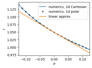
Fig. 6.12 Compressing a disc with an isotropic growth factor