10.1.2. Drums getting exited by a guitar
A band has a rest during rehearsal. As usual, the guitar guy cannot resist to play. By the incident sound wave, the drums are put into motion. We solve the drum exitation height \(h\) by a driven damped wave equation on a circular membrane, where we assume axisymmetric modes only, i.e.
where \(\omega=2\pi f\) is the frequency of the guitar sound incidenting as planar wave with a forcing amplitude of \(F\). \(c\) depends on the drum and the surrounding gas and \(\delta\) is a damping coefficient. We demand that \(h(r=R)=0\) at the radius \(R\) of the drum.
As usual, we start by the drum equation in a coordinate system indepedent weak formulation:
from pyoomph import *
from pyoomph.expressions import *
from pyoomph.expressions.units import *
# Load tools for periodic driving response and text file output
from pyoomph.utils.periodic_driving_response import *
from pyoomph.utils.num_text_out import *

# Driven damped wave equation
class DrumEquation(Equations):
    def __init__(self,c,damping,driving):
        super().__init__()
        self.c,self.damping,self.driving=c,damping,driving

    def define_fields(self):
        # Must be formulated first order here
        self.define_scalar_field("h","C2",testscale=scale_factor("temporal")**2/scale_factor("h"))
        self.define_scalar_field("hdot","C2",scale=scale_factor("h")/scale_factor("temporal"),testscale=scale_factor("temporal")/scale_factor("h"))

    def define_residuals(self):
        h,h_test=var_and_test("h")
        hdot,hdot_test=var_and_test("hdot")
        self.add_weak(partial_t(h)-hdot,hdot_test)
        self.add_weak(partial_t(hdot)+self.damping*hdot-self.driving,h_test)
        self.add_weak(self.c**2*grad(h),grad(h_test))
For the problem, we just define it on a line mesh in axisymmetric coordinates, which are indeed axisymmetric polar coordinates. Thereby, only axisymmetric modes are allowed. Alternatively, one could use a 2d circular Cartesian domain to also allow for nonaxisymmetric modes.
class DrumProblem(Problem):
    def __init__(self):
        super().__init__()
        self.c=60*meter/second
        self.damping=50/second
        self.R_drum=30*centi*meter
        self.driving=meter/second**2 *cos(2*pi*440*hertz*var("time"))

    def define_problem(self):
        self.set_coordinate_system("axisymmetric")
        self+=LineMesh(N=100,size=self.R_drum,name="drum",left_name="center",right_name="rim")
        self.set_scaling(h=1*centi*meter,temporal=0.001*second,spatial=self.R_drum)
        eqs=DrumEquation(self.c,self.damping,self.driving)
        eqs+=DirichletBC(h=0)@"rim"+AxisymmetryBC()@"center"
        eqs+=TextFileOutput()
        self+=eqs@"drum"
The general procedure is the same as before for a simple harmonic oscillator. However, here, we project the response on different Bessel modes:
with DrumProblem() as problem:
        # Create the PeriodicDrivingResponse before the problem is initialized
        pdr=PeriodicDrivingResponse(problem)

        F=10*meter/second**2 # Driving amplitude, does not really matter, will cancel out in the normalized response
        problem.driving=F*pdr.get_driving_mode() # means F*cos(omega*t)

        # solve for a stationary state
        problem.solve()

        # Scan the frequency and write output
        numbessel=10 # Number of Bessel modes to project
        bessel_roots=scipy.special.jn_zeros(0,numbessel)

        outfile=NumericalTextOutputFile(problem.get_output_directory("response.txt"))
        reson_freqs=[float(root*problem.c/problem.R_drum/hertz/(2*pi)) for root in bessel_roots]
        print("RESONANT UNDAMPED FREQS",reson_freqs)
        outfile.header("freq[Hz]",*["mode_"+str(i)+"[mm/(m/s^2)](f={:.4f})".format(reson_freqs[i]) for i in range(numbessel)])

        # Output the resonant undamped frequencies
        freqs=numpy.linspace(1,1000,1000) # Use frequencies f instead of omega
        for response in pdr.iterate_over_driving_frequencies(freqs=freqs,unit=hertz):
            # Get the response as nondimensional data. The response is stored as eigenvector, so we split it in real and imaginary part
            nd_resp_real=problem.get_cached_mesh_data("drum",eigenmode="real",eigenvector=0,nondimensional=True)
            nd_resp_imag=problem.get_cached_mesh_data("drum",eigenmode="imag",eigenvector=0,nondimensional=True)
            # Add interpolators to perform the Bessel projection
            interr=scipy.interpolate.UnivariateSpline(nd_resp_real.get_data("coordinate_x"),nd_resp_real.get_data("h"),k=3,s=0)
            interi=scipy.interpolate.UnivariateSpline(nd_resp_imag.get_data("coordinate_x"),nd_resp_imag.get_data("h"),k=3,s=0)
            # Calculate the Bessel decomposition of the response
            bessel_data=[]
            for i in range(numbessel):
                bess_proj=lambda r : r*scipy.special.j0(bessel_roots[i]*r)*(interr(r)+1j*interi(r))
                numer=scipy.integrate.quad(bess_proj,0,1,complex_func=True)[0] # Integrate BBessel projection
                denom=1/2*scipy.special.j1(bessel_roots[i])**2 # Denominator of the Fourier-Bessel transform
                nd_response_ampl=numpy.absolute(numer/denom)
                dim_response_ampl_by_F=(nd_response_ampl*problem.get_scaling("h")/(milli*meter))/(F/(meter/second**2))
                bessel_data.append(dim_response_ampl_by_F)
            # add a row to the output
            outfile.add_row(pdr.get_driving_frequency()/hertz,*bessel_data)
To obtain the full response data, we can access the eigenvector of the problem. Here, the response is stored in the eigenvector=0. The nondimensional eigenfunction is stored as real and imaginary contribution, which can be accessed by get_cached_mesh_data() for each mesh. Then, cubic interpolators are generated and in the loop, the individual Bessel modes are projected. The result is plotted in Fig. 10.2.
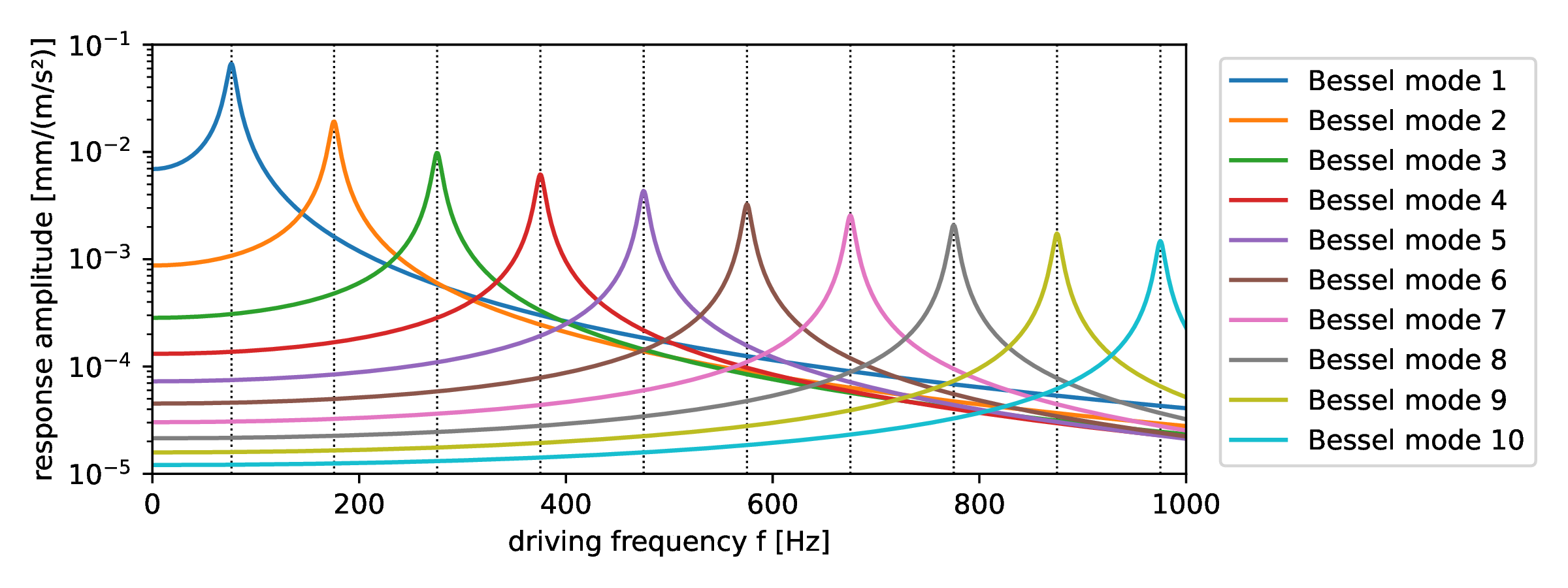
Fig. 10.2 Response of the drum separated into different Bessel modes that fulfill \(h(r=R)=0\). The dashed lines indicate the analytical eigenfrequencies of the undamped wave equation.