10.1.1. Damped harmonic oscillator

Consider a damped harmonic oscillator with driving, i.e.

\[\begin{aligned} \partial_t^2 y+\delta\partial_t y+\omega_0^2 y = F\cos(\omega t)\,. \end{aligned}\]

Due to the damping, all transients will decay and after some time, the system will converge to the response to the driving frequency \(\omega\), i.e. to

\[\begin{aligned} y=A\cos(\omega t + \varphi) \end{aligned}\]

Here \(A\) is the reponse amplitude and \(\varphi\) is the phase shift with respect to the driving. pyoomph can calculate this response automatically for arbitrary problems, i.e. also complex PDEs on moving meshes. To that end, any potential nonlinearities will be linearized around the stationary solution (here, \(y=0\)). First, we define the harmonic oscillator with arbitrary driving and assemble it in a problem. The oscillator must be written as first order system in time, because eventually, an eigenproblem will be solved:

from pyoomph import *
from pyoomph.expressions import *
from pyoomph.expressions.units import *
# Load tools for periodic driving response and text file output
from pyoomph.utils.periodic_driving_response import *
from pyoomph.utils.num_text_out import *

# Driven damped harmonic oscillator
class DampedHarmonicOscillatorEquations(ODEEquations):
    def __init__(self,omega0,delta,driving):
        super().__init__()
        self.omega0,self.delta,self.driving=omega0,delta,driving

    def define_fields(self):
        # Must be formulated first order here
        self.define_ode_variable("y",testscale=scale_factor("temporal")**2/scale_factor("y"))
        self.define_ode_variable("ydot",scale=scale_factor("y")/scale_factor("temporal"),testscale=scale_factor("temporal")/scale_factor("y"))

    def define_residuals(self):
        y,y_test=var_and_test("y")
        ydot,ydot_test=var_and_test("ydot")
        self.add_weak(partial_t(y)-ydot,ydot_test)
        self.add_weak(partial_t(ydot)+self.delta*ydot +self.omega0**2*y-self.driving,y_test)


class DampedHarmonicOscillatorProblem(Problem):
    def __init__(self):
        super().__init__()
        self.omega0=1/second
        self.delta=0.1/second
        # Default driving
        self.driving=meter/second**2 *cos(0.3/second*var("time"))

    def define_problem(self):
        self.set_scaling(y=2*meter,temporal=1*second)
        eqs=DampedHarmonicOscillatorEquations(self.omega0,self.delta,self.driving)
        eqs+=ODEFileOutput()
        self+=eqs@"oscillator"

The trivial way of getting the response is to just integrate over sufficient long time and extract the response \(A\) and the angle \(\varphi\) from the output, i.e.

with DampedHarmonicOscillatorProblem() as problem:
     # Trivial, but long way: integrate in time, extract response manually from the output
     problem.run(100*second,outstep=0.1*second)

However, with the periodic driving response tool, you can scan the linear response quickly:

# Quick way of scanning
# Create the PeriodicDrivingResponse before the problem is initialized
pdr=PeriodicDrivingResponse(problem)

F=1*meter/second**2 # Driving amplitude, does not really matter, will cancel out in the normalized response
problem.driving=F*pdr.get_driving_mode() # means F*cos(omega*t)

# solve for a stationary state
problem.solve()

# Get the equation index to y
dofindices,dofnames=problem.get_dof_description()
yindex=numpy.argwhere(dofindices==dofnames.index("oscillator/y"))[0,0]

# Factor to absorb the dimensions. We want to have response amplitude divided by driving at the end
response_dim_factor=F/meter

# Scan the frequency and write output
outfile=NumericalTextOutputFile(problem.get_output_directory("response.txt"))
outfile.header("omega[1/s]","(A/F)_num[m/(m/s^2)]","phi_num","(A/F)_ana[m/(m/s^2)]")

omegas=numpy.linspace(0.01,3,300)
for response in pdr.iterate_over_driving_frequencies(omegas=omegas,unit=1/second):
    response_ampl,phi=pdr.split_response_amplitude_and_phase() # nondimensional response amplitude and angle
    omega=pdr.get_driving_omega() # current omega
    # redimensionalize the response amplitude and divide by the driving, afterwards nondimensionalize
    A_num=response_ampl[yindex]*problem.get_scaling("y")/F*response_dim_factor
    # Analytic solution
    A_analytic=1/square_root((problem.omega0**2-omega**2)**2+(problem.delta*omega)**2)*response_dim_factor
    phi_analytic=atan2(-problem.delta*omega,problem.omega0**2-omega**2)
    # outpuf
    outfile.add_row(omega*second,A_num,phi[yindex],A_analytic,phi_analytic)

Before the problem is initialized, we must create a PeriodicDrivingResponse object and attach it to the problem. This one will introduce a nondimensional, undamped harmonic oscillator with a variable angular frequency \(\omega\), i.e. \(\partial_t z+\omega^2 z=0\) to the problem. The method get_driving_mode() gives back \(z\), i.e. internally, we use this auxiliary harmonic oscillator to impose the driving to the harmonic oscillator equation for \(y\). To obtain the response, we first must find the equation number corresponding to \(y\), which can be done by describing the degrees of freedom of the problem with the get_dof_description() and finding the correct index in the degrees of freedom. By iterate_over_driving_frequencies(), we can scan a full range of driving frequencies \(\omega\) in a loop. The response is a complex eigenvector, but it can be split into amplitude and phase by split_response_amplitude_and_phase(). By extracting the right component corresponding to \(y\), we get the amplitude and phase directly, correctly account for any physical dimensions and compare it with the analytical solution in the output. The result is plotted in Fig. 10.1.

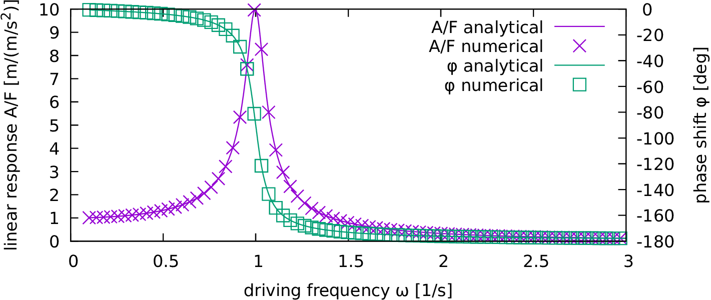
Fig. 10.1 Numerical linear response to a periodic driving with \(F\cos(\omega t)\) of a harmonic oscillator with \(\omega_0=1\) and damping \(\delta=0.1\). The analytical result is also plotted.

Download this example

Download all examples