10.3.2. Path instability of a rising bubble
One particularly powerful feature is the possibility to tackle azimuthal instabilities of rather arbitrary problems defined on moving meshes. Such numerical approaches have been developed only quite recently to investigate e.g. the instability of a rising bubble [4, 29]. Pyoomph does all the cumbersome work of deriving the azimuthal eigenproblem automatically and fully symbolically and generates corresponding C code to fill the mass and Jacobian matrices for these eigenproblems. In the following, we will reproduce the results of [4] in pyoomph.
First of all, we start by defining a rectangular mesh with a circular hole in the center. This hole later represents the bubble. While we could just use the GmshTemplate class to create such a mesh, we prefer to make a structured mesh by manually placing all elements of a coarse mesh, which will be refined during the solution procedure. Read Section 4.3.1 to learn how to create meshes that way. The mesh class itself is skipped here for brevity, but is part of the example code you can download below.
As in [4], we neglect the viscosity and the mass density inside the bubble and nondimensionalize the equations in terms of a Bond number \(Bo=\rho g D^2/\sigma\) and a Galilei number \(Ga=\rho\sqrt{gD^3}/\mu\) (\(D=2R\) is the droplet diameter), where we express the Galilei number by the Bond number via a Morton number \(Mo=g \mu^4/(\rho \sigma^3)\). The Morton number is independent of the bubble size and only depends on the liquid properties and the gravity. In particular, \(Mo=6.2\times 10^{-7}\) holds for DMS-T05 [4], which we consider here. Keeping the Morton number fixed, we can calculate the corresponding Galilei number from the Bond number by \(Ga=(Bo^3/Mo)^{1/4}\). However, the latter expression is problematic if the Bond number becomes negative. By default, pyoomph’s global parameters may attain positive and negative values and therefore, the 4th root will be rather problematic. We therefore inform pyoomph that the Bond number is always a positive parameter. This information will be used in the code generation later on for a good code generation of the 4th root:
class RisingBubbleProblem(Problem):
    def __init__(self):
        super().__init__()
        self.R=0.5
        self.Mo=6.2e-7 # Morton number selects the fluid
        self.Bo=self.define_global_parameter(Bo=0.4) # Bond number, effectively selects the bubble size
         # This helps a lot in reducing the code size: We calculate Ga from Bo with an rational exponent.
         # Since we must separate the real and imaginary part of the azimuthal mode, this would generate a lot of code if Bo could be negative, meaning that Ga could become complex according to the definition
        self.Bo.restrict_to_positive_values()

        self.L_top=15/4 # Far sizes. These are considerably smaller than in the literature
        self.L_bottom=30/4
        self.W=15/4

        self.max_refinement_level=4 # Do not refine more than 4 times (we want to have it fast, not perfectly accurate)
The nondimensionalized equations read
Here, \(U\) is the velocity of the bubble, which is determined by enforcing that the center of mass of the bubble does not move. So we transform into the coordinate system comoving with the bubble as in Section 4.4.7. Also, we have absorbed the hydrostatic pressure in the pressure field \(p\), which leads to the additional axial coordinate \(y\) in the rhs of the pressure acting on the surface. The unknown \(P\) is the bubble pressure which is determined by enforcing a constant nondimensional volume \(4/3\pi R^3\) of the bubble (with \(R=0.5\), i.e. a nondimensional diameter of \(D=1\)). For the volume constraint, we use the divergence theorem trick described in the box in Section 6.7.4. In a similar fashion, the center of mass is calculated by an integration over the surface:
    def define_problem(self):
        Ga=(self.Bo**3/self.Mo)**rational_num(1,4) # Galilei number

        self.set_coordinate_system("axisymmetric")

        self+=StructuredBubbleMesh()  # Add the mesh

        # Assemble the equations: First, output with eigenfunction included
        eqs=MeshFileOutput(operator=MeshDataCombineWithEigenfunction(0))

        # Unknown bubble velocity and bubble pressure (global degrees)
        U,Utest=self.add_global_dof("U")
        P,Ptest=self.add_global_dof("P",equation_contribution=-4/3*pi*self.R**3,initial_condition=8/self.Bo)

        # Bulk equations: Navier-Stokes in the co-moving frame with inertia correction of a potentially accelerating frame
        eqs+=NavierStokesEquations(dynamic_viscosity=1/Ga ,mass_density=1,gravity=vector(0,-1)*partial_t(U),mode="CR")

        # Free surface with the additional pressure of the bubble and the absorbed hydrostatic pressure
        eqs+=NavierStokesFreeSurface(surface_tension=1/self.Bo,additional_normal_traction=P+var("coordinate_y"))@"interface"

        # Constraints fixing the bubble velocity U and the bubble pressure P
        eqs+=WeakContribution(1/2*var("coordinate_y")**2*var("normal_y"),Utest)@"interface"
        eqs+=WeakContribution(-dot(var("coordinate"),var("normal"))/3,Ptest)@"interface"
We still have to add moving mesh equations and some missing boundary conditions. The AxisymmetryBC ensures again the toggling of the \(m\)-dependent boundary conditions for the eigenfunction at \(r=0\). It automatically transfers to e.g. the intersection "interface/axis", where we have to modify e.g. the Lagrange multiplier for the kinematic boundary condition.
        # Boundary conditions
        eqs+=AxisymmetryBC()@"axis"
        eqs+=DirichletBC(mesh_x=self.W,velocity_x=0,velocity_phi=0)@"side"
        eqs+=DirichletBC(mesh_y=-self.L_bottom)@"bottom"
        eqs+=DirichletBC(mesh_y=self.L_top,velocity_x=0,velocity_phi=0)@"top"
        eqs+=EnforcedDirichlet(velocity_y=-U)@"top" # Adjust the far field velocity

        # Add a moving mesh
        eqs+=PseudoElasticMesh()
        # But pin in further away from the bubble to save degrees of freedom
        eqs+=PinWhere(mesh_x=True,mesh_y=True,where=lambda x,y : x**2+y**2>4)

        # Refinement strategy: Max level at the interface
        eqs+=RefineToLevel()@"interface"
        # And also, refine according velocity gradients, both for the base solution and the eigenfunction
        eqs+=SpatialErrorEstimator(velocity=1)

        self+=eqs@"domain"
Optionally, we can process all calculated eigenvectors. Here, we make sure that the average of the mesh displacement at the interface has a zero complex angle. This is possible since eigenvectors can have an arbitrary nonzero multiplicative factor. In particular, it can be complex to rotate the eigenvector with respect to real and imaginary parts. The method process_eigenvectors() is called whenever eigenvectors are calculated. Here, we just call rotate_eigenvectors() to ensure it is rotated the way mentioned above:
    def process_eigenvectors(self, eigenvectors):
        # This function is called whenever the eigenvectors are calculated.
        # Eigenvectors are arbitrary up to a scalar constant.
        # We can multiply it by such a constant that the average x-displacement of the interface mesh has positive real part and zero imaginary part (on average)
        # This is optional, but makes the results more consistent, since the multiplicative constant is otherwise arbitrary
        return self.rotate_eigenvectors(eigenvectors,"domain/interface/mesh_x",normalize_amplitude=0.2,normalize_dofs=True)
The driver code now mainly sets up the problem. In particular, we have to activate again the azimuthal stability analysis. We need a robust complex eigensolver. For that, you have to install a complex variant of the package SLEPc (see Section 2.4).
We then start at some Bond number, relax to the initial state by some transient steps followed by a stationary solve. Then, we create an output file to write the eigenvalues and scan over the Bond number. We solve the eigenproblem using first an initial guess for the eigenvalue (using the shift and target kwargs of solve_eigenproblem()). After the first step, we just use the previously calculated eigenvalue as guess for the next Bond number. We can adapt the mesh based on the eigenfunction using refine_eigenfunction(). It will use the SpatialErrorEstimator added to the problem to refine with respect to jumps in velocity gradients across the elements. Thereby, strong changes in the eigenfunction are better captured:
    with RisingBubbleProblem() as problem:

        # Make sure to get the most optimized code available
        problem.set_c_compiler("system").optimize_for_max_speed()
        # Use SLEPc for the eigenvalue problem, use MUMPS as linear solver, since we have constraints.
        # These have a zero diagonal and give problems in the default LU decomposition of PETSc
        problem.set_eigensolver("slepc").use_mumps()

        # Setup the problem for azimuthal stability analysis. We don't use the analytic Hessian, since we don't do any bifurcation tracking
        # This saves some code generation and compilations time
        problem.setup_for_stability_analysis(azimuthal_stability=True,analytic_hessian=False)

        # Settings
        problem.Mo=6.2e-7 # Morton number selects the fluid
        problem.Bo.value=3 # Start at Bo=3
        BoMax=10 # Maximum Bond number
        dBond=0.25 # Step size in Bond number
        m=1 # Azimuthal mode number
        lambd=-0.1+0.75j # Guess for the eigenvalue

        # Relax to the base state, then solve for the stationary solution
        problem.run(10,startstep=0.1,outstep=False,temporal_error=1)
        problem.solve(max_newton_iterations=20,spatial_adapt=4)

        # Now we can start the eigenanalysis
        outfile=problem.create_text_file_output("m1_instability.txt",header=["Bo","ReLambda","ImLambda"])

        # Scan the branch
        while problem.Bo.value<BoMax:
            # Solve it with a shift-inverted method close to the guess
            problem.solve_eigenproblem(1,azimuthal_m=m,shift=lambd,target=lambd)
            # Refine the mesh according to the eigenfunction and recalculate the eigenproblem
            problem.refine_eigenfunction(use_startvector=True)
            # And update the eigenvalue and the eigenvector guess
            lambd=problem.get_last_eigenvalues()[0] # Update the eigenvalue for the next iteration
            # Store it to the text file
            outfile.add_row(problem.Bo,numpy.real(lambd),numpy.imag(lambd))
            # Output the solution with eigenfunction
            problem.output_at_increased_time()
            # And continue in Bo
            problem.go_to_param(Bo=problem.Bo.value+dBond)
Eventually, we get the eigenvalues shown below, which agree decently with the data of [4]. We can do the same for other liquids and branches described in [4]. Note that our mesh is quite coarse and small in terms of the far field, so one might have to take a finer mesh (using the max_refinement_level) and a larger domain with the properties L_top, L_bottom and W of our problem class. Also note that the plots of the solutions in [4] apparently scale the nondimensional radius, not the diameter to unity. Therefore, the fields have different amplitudes.
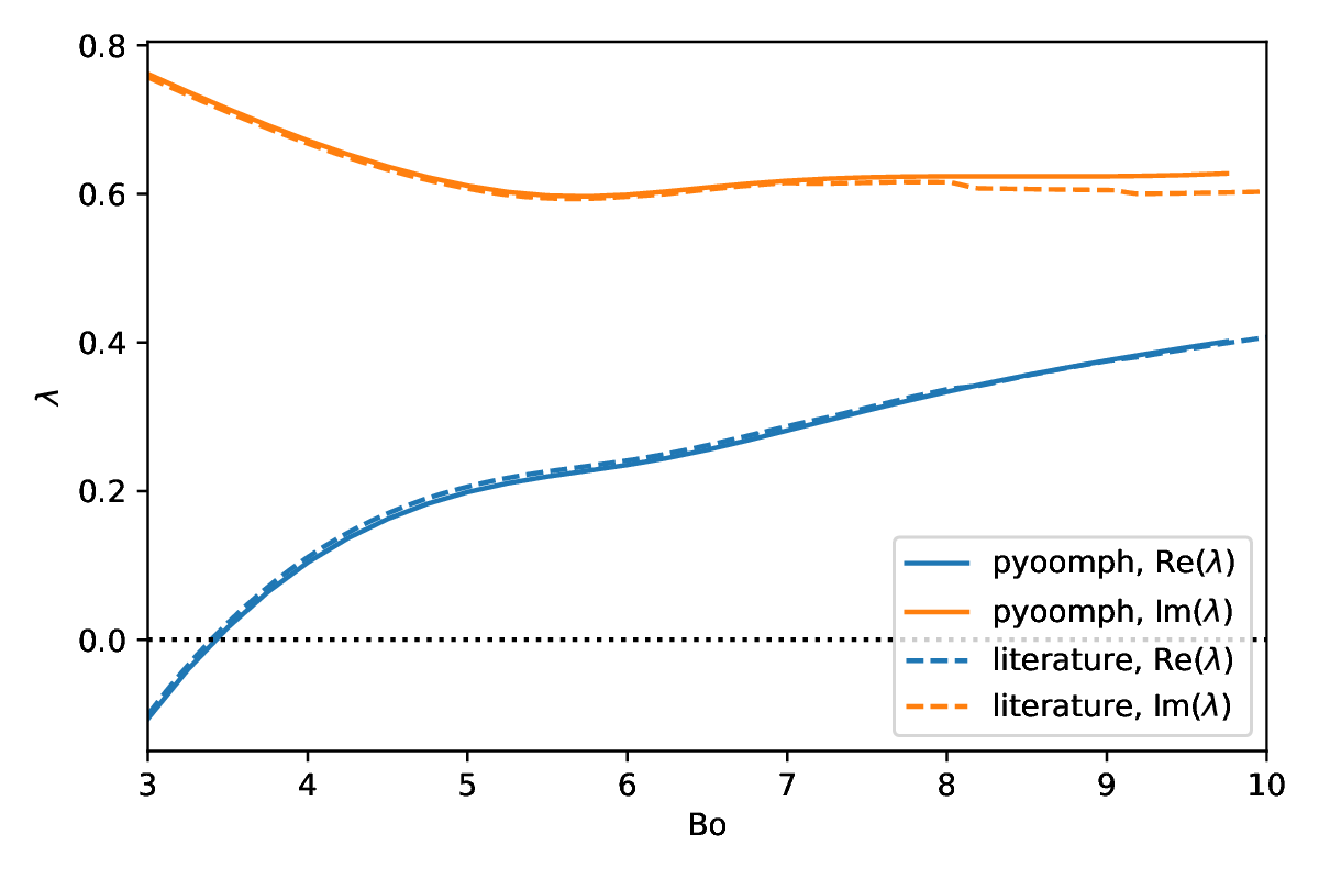
Fig. 10.5 Eigenvalues of the first \(m=1\) instability of a rising bubble with \(Mo=6.2\times 10^{-7}\) (DMS-T05), agreeing well with the literature data. We thank Javier Sierra-Ausin and Jacques Magnaudet for providing the data of their paper.
We can also generate a movie of the instability. Please refer to Section 11.4 for a tutorial on this.
Eigendynamics at \(Bo=4\)