3.12.3. Stability of orbits
As stationary solutions, periodic orbits can exhibit different kinds of stabilities. In the discussed Lorenz system, we only found unstable orbits, but how to prove that they are indeed unstable? As usual, stability can be defined by the linearized dynamics around the state of interest, here the orbit.
Recalling (3.21), a linearization around the orbit \(\vec{x}(t)\) corresponds to the solution
Here, \(\mathbf{J}_0(\vec{x})\) is the Jacobian of the time-independent residual \(\vec{R}_0(\vec{x})\) and \(\vec{v}(t)\) is the linear perturbation of the orbit. After one period, we do not necessarily end up at the very same point, i.e. in general \(\vec{v}(t+T)\neq \vec{v}(t)\). Instead, we generically end up at another point, which is expressed by the so-called Floquet multiplier \(\lambda\). Floquet theory tells us that such solutions \(\vec{v}(t)\) with corresponding values of \(\lambda\) exist, which resemble the conventional eigenvectors and -values used for the stability of stationary solutions, although there are some differences as detailed in the following. Due to linearity, a second turn along the orbit will end up at \(\vec{v}(t+2T)=\lambda^2 \vec{v}(t)\) and (as long as the perturbation remains small) a multiplicator of \(\lambda^n\) after \(n\) periods. Obviously, an orbit is stable if all Floquet multipliers (which are in general complex-valued) satisfy \(|\lambda|<1\). However, there is always a Floquet multiplier \(\lambda=1\) present in the system, which corresponds to the shift invariance in time. The corresponding perturbation is just \(\vec{v}=\partial_t\vec{x}\), i.e. if we just start our perturbation somewhere else in time, we will end up shifted as well after a period of \(T\).
Pyoomph can calculate Floquet multipliers, which is demonstrated in the following on the basis of the Langford ODE system. This one reads with suitable parameters [25]:
For \(\mu>1.683\), perfectly circular orbits can be found which change the stability from stable to unstable at \(\mu=2\) [25].
Implementing the equation and setting up the problem is again trivial:
#See https://arxiv.org/abs/2407.18230v1
class LangfordSystem(ODEEquations):
     def __init__(self,mu):
             super(LangfordSystem,self).__init__()
             self.mu=mu

     def define_fields(self):
             self.define_ode_variable("x","y","z")

     def define_residuals(self):
             x,y,z=var(["x","y","z"])
             xrhs=(self.mu-3)*x-0.25*y+x*(z+0.2*(1-z**2))
             yrhs=(self.mu-3)*y+0.25*x+y*(z+0.2*(1-z**2))
             zrhs=self.mu*z-(x**2+y**2+z**2)
             residual=(partial_t(x)-xrhs)*testfunction(x)
             residual+=(partial_t(y)-yrhs)*testfunction(y)
             residual+=(partial_t(z)-zrhs)*testfunction(z)
             self.add_residual(residual)


class LangfordProblem(Problem):
    def __init__(self):
         super().__init__()
         self.mu=self.define_global_parameter(mu=1.6)

    def define_problem(self):
        eqs=LangfordSystem(self.mu)
        eqs+=ODEFileOutput()
        self.add_equations(eqs@"langford")

    def get_analytical_nontrivial_floquet_multiplier(self):
        # Calculate the analytical nontrivial Floquet multiplier
        muv=self.mu.value
        z=2.5*(1-numpy.sqrt(0.8*muv-1.24))
        r=numpy.sqrt(z*(muv-z))
        exponent=(muv-2*z+numpy.emath.sqrt((muv-2*z)**2-8*r*(r-0.4*r*z)))/2
        T=4*2*numpy.pi
        multiplier=numpy.exp(exponent*T)
        if numpy.imag(multiplier)<0:
            multiplier=numpy.conjugate(multiplier) # We always consider the one with positive imaginary part
        return multiplier
Note how we also provide a function to calculate the analytical nontrivial Floquet multiplier [25], i.e. a complex Floquet multiplier which is not the trivial one \(\lambda=1\).
We will then again find the Hopf bifurcation, switch to the orbit and continue in the parameter \(\mu\). But at each continuation step, we also calculate the Floquet multipliers and write the non-trivial one (along with the corresponding analytical solution) to the output:
with LangfordProblem() as problem:
   # Use again an analytic Hessian for the determination of the first Lyapunov coefficient
   problem.setup_for_stability_analysis(analytic_hessian=True)
   # We also need the SLEPc eigensolver here
   problem.set_eigensolver("slepc").use_mumps()

   problem+=InitialCondition(x=0.01,z=1.1)@"langford"  # Some non-trivial initial position

   # Find the Hopf bifurcation as usual
   problem.solve()
   problem.solve_eigenproblem(3)
   problem.activate_bifurcation_tracking("mu")
   problem.solve()

   # Output file to compare the numerical and analytical Floquet multipliers
   floquet_output=problem.create_text_file_output("floquet.txt",header=["mu","num_real","num_imag","ana_real","ana_imag"])

   # Switch again to the orbits originating from the Hopf bifurcation
   with problem.switch_to_hopf_orbit(NT=50,order=3) as orbit:
           ds=orbit.get_init_ds()
           maxds=ds*100 # Limit the maximum step size
           while problem.mu.value<2.05:
                   ds=problem.arclength_continuation("mu",ds,max_ds=maxds)
                   F=orbit.get_floquet_multipliers(n=3,shift=3) # Calculate some Floquet multipliers
                   # However, not always three multipliers are found. We have to consider the cases
                   if len(F)==3:
                           # Three multipliers found: The trivial one and two complex conjugate ones
                           F=numpy.delete(F,numpy.argmin(numpy.abs(F-1)))
                           nontrivial_floquet=F[0] # Take one of the complex conjugate multipliers
                   elif len(F)==2:
                           # Only two multipliers found: The trivial one and one real one
                           F=numpy.delete(F,numpy.argmin(numpy.abs(F-1)))
                           nontrivial_floquet=F[0] # Take the remaining multiplier
                   else:
                           # Only one multiplier found: The trivial one
                           nontrivial_floquet=0 # The others are then very close to 0

                   if numpy.imag(nontrivial_floquet)<0:
                           # conjugate a multiplier with negative imaginary part
                           nontrivial_floquet=numpy.conjugate(nontrivial_floquet)

                   # Output the orbit
                   odir="orbit_{:.3f}".format(problem.mu.value)
                   orbit.output_orbit(odir)

                   # Write to output for comparison
                   floq_ana=problem.get_analytical_nontrivial_floquet_multiplier()
                   floquet_output.add_row(problem.mu, nontrivial_floquet.real,nontrivial_floquet.imag,floq_ana.real,floq_ana.imag)
Floquet multipliers can be calculated via the method get_floquet_multipliers() of the PeriodicOrbit class. The internals work analogously to the way proposed in Ref. [19]. However, multipliers close to zero will be discarded. The usually do not give any information on the stability anyways. We carefully have to select the interesting Floquet multiplier and write it to the output. As depicted in Fig. 3.19, the results agrees well with the analytical Floquet multiplier.
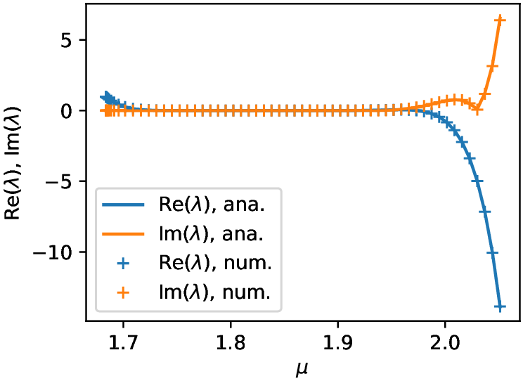
Fig. 3.19 Floquet multipliers of the Langford ODE system
Since the Floquet multipliers at \(\mu=2\) cross the stability condition \(|\lambda|=1\) by a complex-conjugated pair, this corresponds to a Neimark-Sacker bifurcation. The orbit becomes unstable to a torus. We can check this by performing time integration. The moment we leave the with statement of the orbit, pyoomph will initialize the degrees of freedom to the starting point of the orbit. A trivial run() statement will then perform a time integration along the orbit. However, if we start at \(\mu>2\) (here e.g. \(\mu=2.005\)), it will be unstable and we can see the torus developing. We just have to replace the orbit loop by (i.e. the code after solving for the Hopf bifurcation) by:
with problem.switch_to_hopf_orbit(NT=50,order=3) as orbit:
        ds=orbit.get_init_ds()
        maxds=ds*100 # Limit the maximum step size
        problem.go_to_param(mu=2.005,startstep=ds,max_step=maxds,call_after_step= lambda ds: orbit.output_orbit("orbit_at_mu_"+str(problem.mu.value)))
        T=orbit.get_T() # Get the period
        NT=orbit.get_num_time_steps() # Get the number of time steps
        dt=T/NT # And calculate a good time step

# Running a transient integration starting on the orbit
problem.run(40*T,outstep=dt/4)

Fig. 3.20 Stable orbits (color-coded by \(\mu\)) and time integration at \(\mu=2.005\) (black) showing the unstable dynamics building a torus. Also, the path of the Floquet multipliers as function of \(\mu\) is shown.