4.4.8. Using a discontinuous pressure - Crouzeix-Raviart elements

So far, we have only addressed the continuous spaces "C1" and "C2". Pyoomph has additional finite element spaces which can be used. In particular for solving flow problems, there is - besides the Taylor-Hood element - the Crouzeix-Raviart element [8]. In fact, a Taylor-Hood approximation (i.e. using "C2" for the velocity and "C1" for the pressure) does guarantee to fulfill the continuity equation in each element, but only globally on the entire domain, i.e. in- and outfluxes through domain boundaries are balanced, but not necessarily in each element.

The reason for that can be found in the continuous pressure space. The pressure acts as a Lagrange multiplier field enforcing the incompressibility. However, since the degrees of freedom of the pressure are shared by neighboring elements, the incompressibility is not enforced on a elemental basis. To achieve this, one must make sure that all pressure degrees of freedom are associated with a single element, which means that the pressure field may become discontinuous across the elements. While there are several choices for Crouzeix-Raviart elements, we will focus on the same as oomph-lib provides, where the pressure is represented by an affine linear function in each element.

In pyoomph, the discontinuous space "DL" introduces exactly these degrees of freedom, i.e. in each element, the pressure field will follow an affine linear relation

(4.20)\[p^\text{el}(\vec{x})=\vec{a}^\text{el}\cdot(\vec{x}-\vec{x}_\text{c}^\text{el})+b^\text{el}\]

where \(\vec{a}^\text{el}\) accounts for the slopes of the pressure within the element, \(\vec{x}_\text{c}^\text{el}\) is the center of the element and \(b^\text{el}\) is the offset to account for the degree of freedom in the absolute pressure. The superscript \({}^\text{el}\) is used to indicate that these quantities change when moving to the next element, while they are constants within each element. As a nota bene, pyoomph also has the discontinuous space "D0", which is just constant in each element, i.e. (4.20) with \(\vec{a}^\text{el}=0\). For an illustration, of the continuous spaces "C1" and "C2" and the discontinuous spaces "DL" and "D0", please refer to Fig. 4.21.

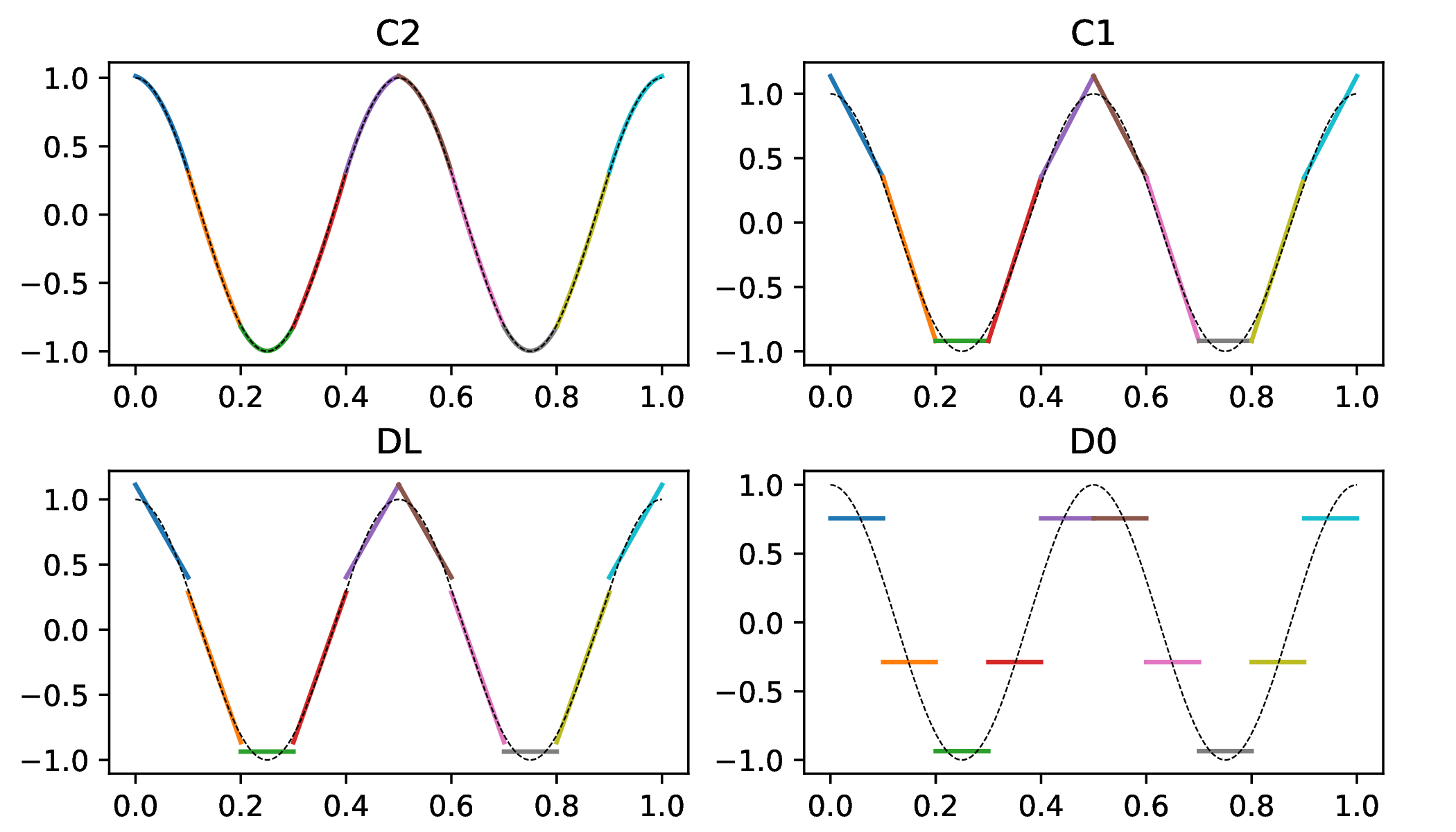
Fig. 4.21 Approximations of \(\cos(4\pi x)\) (dashed line) by different spaces. The different colors correspond to the elements.

The Crouzeix-Raviart elements of oomph-lib combine the "C2" space for the velocity with the "DL" space for the pressure. This is at least true for quadrilateral elements, whereas for triangular elements, the velocity would be over-constrained by the incompressibility enforced on the "DL" space. For these elements, a cubic bubble velocity degree must be added to the "C2" space. This additional bubble degree is located in the center of the triangular element (see Fig. 4.22). Likewise, a three-dimensional tetrahedral element must be enriched by bubbles.

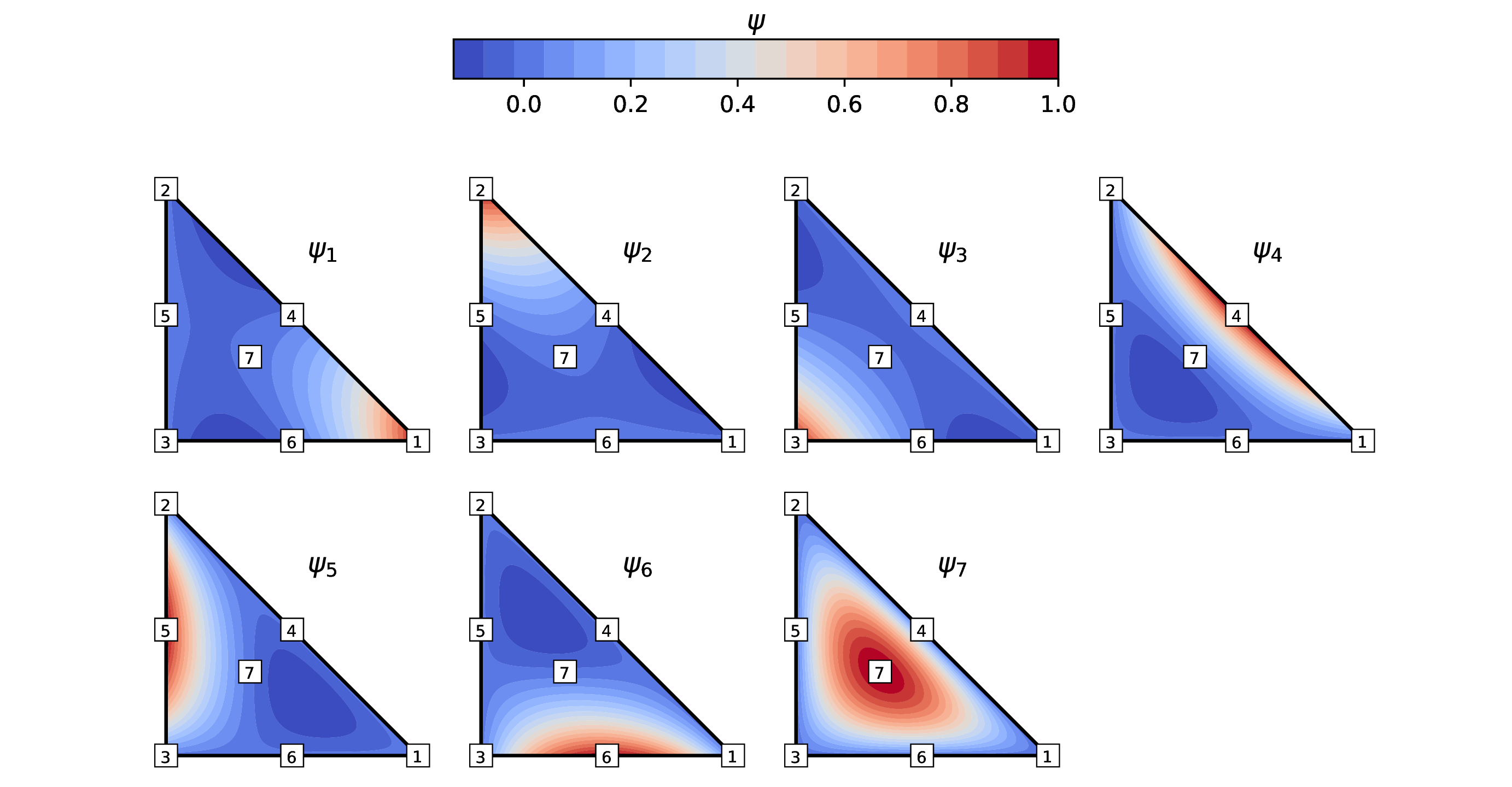
Fig. 4.22 Bubble-enriched triangular element, i.e. showing the space "C2TB".

Since pyoomph separates the spaces and the elements, an additional space "C2TB" is introduced, which is "C2" on each quadrilateral element, but will enrich each triangular or tetrahedral element by bubble degrees. Hence, we can use the Crouzeix-Raviart elements on both quadrilateral and triangular elements, by just passing the combination "C2TB", "DL" to the Stokes problem with space selection from Section 4.4.2:

from stokes import *

if __name__ == "__main__":
    # Create a Stokes problem with viscosity 1, on a Crouzeix-Raviart element
    with StokesSpaceTestProblem(1.0, "C2TB", "DL") as problem:
        problem.solve()  # solve and output
        problem.output()

The benefit of Crouzeix-Raviart elements is the elementwise valid continuity equation, but it comes at the price of an increased number of degrees of freedom.

Warning

When using MeshFileOutput for the discontinuous space "DL", it will not show the gradients, but only the value at the centroid of the element. This is due to the fact that VTU files do not support cell data that varies in space.

Warning

Continuous spaces are directly transferred to the interfaces. Thereby, we can access the velocity on the interface by var_and_test("velocity") on an InterfaceEquations class, as e.g. in the example in Section 4.4.6. Discontinuous fields, like the pressure here, are internally stored in the bulk elements and hence cannot be accessed directly by the attached interfaces, but you can access it by e.g. var_and_test("pressure",domain=self.get_parent_domain()) on interfaces.

For the same reason, you cannot set DirichletBC terms for discontinuous fields at interfaces. While usually you do not set DirichletBCs for the pressure, this can be problematic for the case discussed in Section 4.4.4, where one degree of the pressure had to be eliminated to remove the null space. To that end, the predefined StokesEquations in pyoomph.equations.navier_stokes have a function to fix one pressure degree for both cases, Taylor-Hood and Crouzeix-Raviart elements. See stokes_pressure_fix.py for an example how to use it.

Tip

oomph-lib covers the Taylor-Hood and the Crouzeix-Raviart elements in the example https://oomph-lib.github.io/oomph-lib/doc/navier_stokes/driven_cavity/html/index.html.