5.1.1. Simple wave equation in one dimension

Let us start with a simple wave equation

(5.1)\[\partial_t^2 u-c^2\nabla^2 u=0\,.\]

Upon multiplication with the test function \(w\) and partial integration, one obtains the weak form

(5.2)\[\left(\partial_t^2 u,w\right)+\left(c^2\nabla u,\nabla w\right)-\left\langle c^2\nabla u\cdot\vec{n},w \right\rangle =0\,.\]

In pyoomph, we just can use partial_t() for the time derivative and do the spatial part as before in Section 4. For the bulk contributions, i.e. the \((\cdot,\cdot)\) terms, we write again a Equations class:

from pyoomph import *
from pyoomph.expressions import *


class WaveEquation(Equations):
     def __init__(self,c=1):
             super(WaveEquation, self).__init__()
             self.c=c # speed

     def define_fields(self):
             self.define_scalar_field("u","C2")

     def define_residuals(self):
             u,w=var_and_test("u")
             self.add_residual(weak(partial_t(u,2),w)+weak(self.c**2*grad(u),grad(w)))

It is essentially the same approach as in Section 3. The problem class could read as follows

class WaveProblem(Problem):
     def __init__(self):
             super(WaveProblem, self).__init__()
             self.c=1 # speed
             self.L=10 # domain length
             self.N=100 # number of elements

     def define_problem(self):
             # interval mesh from [-L/2 : L/2 ] with N elements
             self.add_mesh(LineMesh(N=self.N,size=self.L,minimum=-self.L/2))

             eqs=WaveEquation() # equation
             eqs+=TextFileOutput() # output
             eqs+=DirichletBC(u=0)@"left" # fixed knots at the end points
             eqs+=DirichletBC(u=0)@"right"

             # Initial condition
             x,t=var(["coordinate_x","time"])
             #u_init=exp(-x**2) # This has no initial motion, i.e. partial_t(u)=0
             u_init=exp(-(x-self.c*t)**2) # This one moves initially to the right
             eqs+=InitialCondition(u=u_init) # setting the initial condition

             self.add_equations(eqs@"domain") # adding the equation

if __name__=="__main__":
     with WaveProblem() as problem:
             problem.run(20,outstep=True,startstep=0.1)

Note how the initial condition u_init depends on time t, which is bound by var("time") again. Thereby, we ensure that we have a traveling wave solution. Besides the initial condition \(u(x,t{=}0)\), the additionally required first derivative \(\partial_t u(x,t{=}0)\) is automatically evaluated. Indeed the result is, as expected, a traveling wave which is reflected at the boundaries, cf. Fig. 5.1. Without specifying the time dependency of the initial condition, \(\partial_t u(x,t{=}0)=0\) would hold, yielding a different solution.

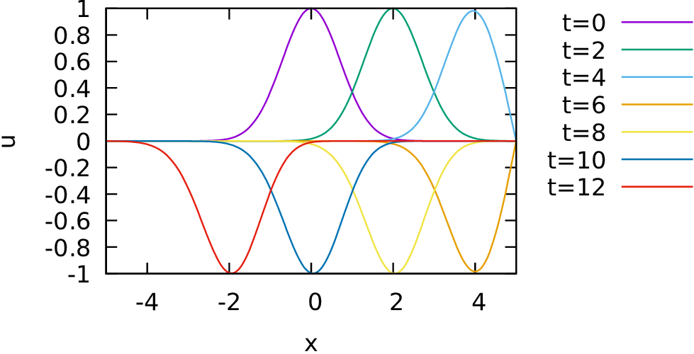
Fig. 5.1 Traveling wave solution, which is reflected at the boundaries.

Without the DirichletBC(u=0) terms, the \(\langle \cdot, \cdot \rangle\) terms in (5.2) would become relevant. Since we do not add any contributions at the boundaries by some InterfaceEquations or NeumannBC, the term \(\langle c^2\nabla u\cdot\vec{n},w \rangle\) is zero. This can only hold for arbitrary \(w\), if \(\partial_x u=0\). Thereby, the wave will have free ends on both sides. The wave gets reflected, but without changing sign.

Download this example

Download all examples