5.1.2. Playing drums - Wave equation on a circular domain
Since pyoomph supports the definition of the Equations class independently of the number of spatial dimensions and coordinate systems, the same wave equation can be reused to solve it on other domains. Let us just solve the equation on a circular domain with radius \(R\) now. The analytical result is well known and is expressed as a Fourier-Bessel series:
Here, \((r,\theta)\) are the polar coordinates and \(\alpha_m\) and \(\beta_m\) are amplitudes of the polar modes of index \(m\). \(A_mn\) is the amplitude of the radial mode \((m,n)\), where \(J_m\) is the Bessel function of the first kind. \(\lambda_{mn}\) is the \(n^{\mathrm{th}}\) positive root of \(J_m\).
pyoomph does not have the Bessel functions implemented, but the Python package scipy does. However, since pyoomph compiles the equations to C code, we must wrap the scipy implementation of the Bessel functions in a CustomMathExpression callback function:
from wave_eq import * # Import the wave equation from the previous example
from pyoomph.meshes.simplemeshes import CircularMesh # Import the circle mesh

# Required for Bessel functions
import scipy.special


# Expose the Bessel function from scipy to pyoomph
class BesselJ(CustomMathExpression):
	def __init__(self,m):
		super(BesselJ,self).__init__()
		self.m=m # index of the Bessel function

	def eval(self,arg_arry):
		return scipy.special.jv(self.m,arg_arry[0]) # Return the scipy result
The problem class can then use the BesselJ class to set up a single angular mode \(m\) with some excited radial modes \((m,n)\) as InitialCondition:
class WaveProblemCircularMesh(Problem):
	def __init__(self):
		super(WaveProblemCircularMesh, self).__init__()
		self.c=1 # speed
		self.R=10 # domain length
		self.m=3 # angular mode
		self.alpha=1 # coefficient of cos
		self.beta=0 # coefficient of sin
		self.radial_amplitudes=[1,-0.4,0.8] # radial amplitudes of R_mn

	def define_problem(self):
		self.add_mesh(CircularMesh(radius=self.R)) # Circular mesh

		eqs=WaveEquation(self.c) # equation
		eqs+=MeshFileOutput() # output
		eqs+=DirichletBC(u=0)@"circumference" # fixed knots at the rim
		eqs+=RefineToLevel(4) # the CircularMesh is by default coarse, refine it 4 times

		# Initial condition
		x, y = var(["coordinate_x","coordinate_y"]) # Cartesian coordinates
		r, theta = square_root(x**2+y**2), atan2(y,x)  # polar coordinates
		J_m=BesselJ(self.m) # bind the Bessel function with integer index m
		bessel_roots=scipy.special.jn_zeros(self.m, len(self.radial_amplitudes)) # get the Bessel roots lambda_mn

		Theta=self.alpha*cos(self.m*theta)+self.beta*sin(self.m*theta) # angular solution
		R=sum([A*J_m(r*lambd/self.R) for A,lambd in zip(self.radial_amplitudes,bessel_roots)]) # radial solution
		eqs+=InitialCondition(u=Theta*R) # setting the initial condition

		self.add_equations(eqs@"domain") # adding the equation


if __name__=="__main__":
	with WaveProblemCircularMesh() as problem:
		problem.run(20,outstep=True,startstep=0.1)
First of all, we use the CircularMesh, which is very coarse by default. However, since we add a RefineToLevel object to the equations of the circular domain, the mesh will be refined (\(4\) times here). The initial condition is then assembled to match a single angular mode \(m\) with a few excited radial modes \((m,n)\). The amplitudes can be controlled by the alpha, beta and radial_amplitudes properties of the Problem class. We use scipy‘s functionality to find the first roots of \(J_m\) and eventually pass the assembled initial excitation as InitialCondition.
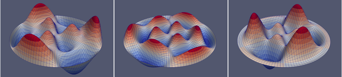
Fig. 5.2 Numerically obtained solution of the wave equation on a circular domain at three different time instants.