5.2.1. Naive implementation
Let us first ignore this complication and implement the equation naively. We will add a flag advection_in_partial_integration to choose between both different weak forms of the advection term:
from pyoomph import *
from pyoomph.expressions import *


class ConvectionDiffusionEquation(Equations):
	def __init__(self,u,D,advection_in_partial_integration,space="C2"):
		super(ConvectionDiffusionEquation, self).__init__()
		self.u=u # advection velocity
		self.D=D # diffusivity
		self.space=space # space of the field c
		self.advection_in_partial_integration=advection_in_partial_integration # Which weak form to use

	def define_fields(self):
		self.define_scalar_field("c",self.space) # The scalar field to advect

	def define_residuals(self):
		c,phi=var_and_test("c")
		# Advection either intergrated by parts or not
		advection=-weak(self.u*c,grad(phi)) if self.advection_in_partial_integration else weak(div(self.u*c),phi)
		# TPZ or MPT time stepping can be of advantage compared to BDF2
		self.add_residual(time_scheme("TPZ",weak(partial_t(c),phi)+advection+weak(self.D*grad(c),grad(phi))))
Depending on the value of advection_in_partial_integration, we either use (5.3) or (5.4) for the weak form. Furthermore, we changed the time stepping from the default "BDF2" to "TPZ", which can be of advantage (cf. Section 3.6.3 for time stepping methods).
As a problem class, we use a bump which is swirled around by one period. When the diffusivity is low, we expect the bump to be only slightly smaller in amplitude and only slightly coarser due to diffusion. The problem class hence reads:
class ConvectionDiffusionProblem(Problem):
	def __init__(self):
		super(ConvectionDiffusionProblem, self).__init__()
		self.u=2*pi*vector([-var("coordinate_y"),var("coordinate_x")]) # Circular flow, one rotation at t=1
		self.D=0.001 # diffusivity
		self.L=1 # size of the mesh
		self.N=4 # number of elements of the coarsest mesh in each direction
		self.max_refinement_level=5 # max refinement level
		self.advection_in_partial_integration=False # which weak form to choose

	def define_problem(self):
		self.add_mesh(RectangularQuadMesh(lower_left=-self.L/2,size=self.L,N=self.N))

		eqs=ConvectionDiffusionEquation(self.u,self.D,self.advection_in_partial_integration)
		eqs+=MeshFileOutput() # output

		# use a bump as initial condition
		bump_pos=vector([-self.L/5,0]) # center pos of the bump
		bump_width=0.005*self.L # width of the bump
		bump_amplitude=1 # amplitude of the bump
		xdiff=var("coordinate")-bump_pos # difference between coordinate and bump center
		bump=bump_amplitude*exp(-dot(xdiff,xdiff)/bump_width) # Gaussian bump
		eqs+=InitialCondition(c=bump)

		# Set the boundaries to 0
		for b in ["top","left","right","bottom"]:
			eqs+=DirichletBC(c=0)@b

		# Errors: We evaluate the jumps in the gradients of c at the element boundaries, i.e. when crossing to the next element
		# this is not only done at the current time step, but also on the previous one
		error_fluxes=[grad(var("c")),evaluate_in_past(grad(var("c")))]
		eqs+=SpatialErrorEstimator(*error_fluxes)

		self.add_equations(eqs@"domain") # adding the equation
The most interesting thing here is that we can also define a SpatialErrorEstimator based on history values. Instead of passing keyword arguments, we can also pass positional arguments to the SpatialErrorEstimator. The error estimator requires gradients, but these can also be evaluated at previous time steps. This ensures that the wake remains more finely resolved.
The run code is again simple:
if __name__=="__main__":
	with ConvectionDiffusionProblem() as problem:
		problem.advection_in_partial_integration=True # Can also set it to false
		problem.D=0.0001 # diffusivity
		problem.run(1,outstep=0.01,maxstep=0.0025,spatial_adapt=1,temporal_error=1)
Using outstep=0.01 in the run(), we will get 100 outputs, but due to maxstep=0.0025, we solve at least 4 times per output. spatial_adapt=1 will perform, as usual, one spatial adaption per solve, whereas temporal_error=1 just ensures that the time step gets reduced when it does not converge.
Results at different times are depicted in Fig. 5.4.
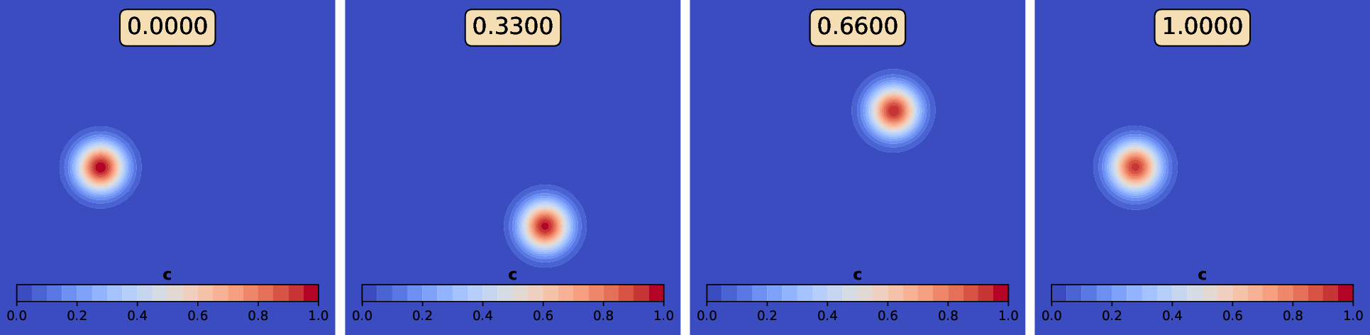
Fig. 5.4 Advecting a bump with low diffusivity.