10.2.1. Droplet detaching by gravity
Consider a droplet hanging at the bottom of a horizontal wall, where the contact line is pinned at some fixed radius \(R\). What is the maximum volume \(V_\text{c}\) the droplet can assume before it pinches off due to gravity? Obviously, if the volume is less, \(V<V_\text{c}\), the droplet will assume some stationary state which can be calculated by the Young-Laplace equation. If the volume exceeds \(V>V_\text{c}\), this stationary state of a hanging droplet will either lose its stability or this solution will even cease to exist (fold bifurcation). At \(V=V_\text{c}\) an eigenvalue of the stationary solution must cross \(0\), at least the real part. Since the stationary solution has vanishing velocity and also there is no instrinsic time scale, the critical volume \(V_\text{c}\) will be independent on the Reynolds number, but of course the balance of gravity and surface tension will enter, i.e. the Bond number
Even if inertia does not enter for the critical volume \(V_\text{c}(\operatorname{Bo})\), we require the time derivative of the velocity to appear in the mass matrix for the eigenvalue determination. And, of course, the dynamical behavior of the pinch-off is strongly dependent on the liquid properties, expressed e.g. in the Reynolds, Ohnesorge or capillary number, but this is irrelevant for the determination of \(V_\text{c}(\operatorname{Bo})\).
For more details please refer to [16].
We start by a hemispherical droplet with \(R=1\) at \(\operatorname{Bo}=0\). To that end, we create the following mesh:
from pyoomph import *
from pyoomph.equations.navier_stokes import * # Navier-Stokes for the flow
from pyoomph.equations.ALE import * # Moving mesh equations
from pyoomph.meshes.remesher import Remesher2d # Remeshing
from pyoomph.utils.num_text_out import NumericalTextOutputFile # Tool to write a file with numbers

# Make a mesh of a hanging hemispherical droplet with radius 1
class HangingDropletMesh(GmshTemplate):
    def define_geometry(self):
        self.default_resolution=0.05
        self.mesh_mode="tris"
        self.create_lines((0,-1),"axis",(0,0),"wall",(1,0))
        self.circle_arc((0,-1),(1,0),center=(0,0),name="interface")
        self.plane_surface("axis","wall","interface",name="droplet")
        self.remesher=Remesher2d(self) # attach a remesher
It is rather trivial, just three points, an axis of symmetry, a wall at the top and a circle segment as interface. We also add a remesher, since remeshing is required due to large mesh deformations.
The problem class itself starts also quite simple, we just add the two parameters \(\operatorname{Bo}\) and the volume \(V\) with good starting values, i.e. without gravity and with the volume of the hemispherical initial mesh (in axisymmetry), so that the parameters agree with the initial stationary solution. We then add NavierStokesEquations with the correct bulkforce. For the mass density and dynamic viscosity, any numerical value can be taken (\(>0\)). It does not change the result since the stability is determined by a balance of surface tension and gravity alone. Also the boundary conditions are added, i.e. axisymmetry at the axis, no-slip and fixed coordinates at the wall, as well as a free surface (with unity surface tension due to non-dimensionalization with the Bond number). Also, the detection of required remeshing is added with default parameters:
class HangingDropletProblem(Problem):
    def __init__(self):
        super().__init__()
        # Initially no gravity
        self.Bo=self.define_global_parameter(Bo=0)
        # Initial volume of a hemispherical droplet with radius R=1
        self.V=self.define_global_parameter(V=2*pi/3)

    def define_problem(self):
        self.set_coordinate_system("axisymmetric") # axisymmetry
        self+=HangingDropletMesh() # Add the mesh

        # Bulk equations: Navier-Stokes + Moving Mesh
        eqs=MeshFileOutput() # Paraview output
        # Mass density can be set arbitrarly with the same results. But must be >0 to get a du/dt -> mass matrix
        eqs+=NavierStokesEquations(dynamic_viscosity=1,mass_density=1,bulkforce=self.Bo*vector(0,-1))
        eqs+=LaplaceSmoothedMesh()

        # Boundary conditions:
        eqs+=(DirichletBC(mesh_y=0,mesh_x=True)+NoSlipBC())@"wall" # static no-slip wall
        eqs+=AxisymmetryBC()@"axis"
        eqs+=NavierStokesFreeSurface(surface_tension=1)@"interface" # free surface

        # Remeshing
        eqs+=RemeshWhen(RemeshingOptions())
As already pointed out in Section 6.6.4, stationary solutions on a moving mesh are problematic, since there are plenty of stationary solutions that do not necessary have the desired volume \(V\). Again, we have to enforce the desired volume \(V\) by adding a Lagrange multiplier which then acts on the pressure:
# For stationary solutions, we must enforce the droplet volume to be the given one
# Add a global Lagrange multiplier -> something like the gas pressure that acts to ensure the volume
# we want to solve p_gas by integral_droplet(1*dx)-Paramter_V=0, so we subtract the symbolic volume parameter
self+=GlobalLagrangeMultiplier(p_gas=-self.V,only_for_stationary_solve=True)@"globals"
p_gas=var("p_gas",domain="globals") # bind the gas pressure
# And rewrite 1*dx=div(x)/3*dx=1/3*x*n*dS, add it to the p_gas equation to complete it
eqs+=WeakContribution(1/3*var("mesh"),var("normal")*testfunction(p_gas))@"interface"
# p_gas must now act somewhere. We just let it act on the contact line, and only if solved stationary
# The kinematic BC at the rest of the interface will adjust accordingly
eqs+=EnforcedBC(pressure=p_gas,only_for_stationary_solve=True)@"interface/wall"

# Add the equation system to the droplet
self+=eqs@"droplet"
Note how we use the trick mentioned in the info box in Section 6.6.4 here to calculate the actual volume \(\int 1 \mathrm{d}V\) by a surface integral. The other surfaces (axis of symmetry and wall) are not required, since \(\vec{x}\cdot\vec{n}=0\). With the Lagrange multiplier, the pressure at the contact line is enforced to the required pressure for the given volume. All other contributions, i.e. the values of the Lagrange multiplier field that enforces the kinematic boundary condition, will adjust accordingly. Also note that we pass the keyword-argument only_for_stationary_solve=True to the GlobalLagrangeMultiplier. With this, both the global Lagrange multiplier and the enforced contact line pressure, will be disabled during any transient solve, where volume enforcing is not required. Thereby, the problem can be used for both stationary solve() and transient run() statements.
The run code to determine the curve is quite simple. We start with:
if __name__=="__main__":
    with HangingDropletProblem() as problem:
        # Calculate the Hessian symbolically/analytically -> faster and more accurate than finite differences
        problem.setup_for_stability_analysis()
        problem.do_call_remeshing_when_necessary=False # Don't auto-remesh. Can be problematic during continuation

        # Increase Bond number towards the bifurcation, do remeshing if necessary during that
        problem.go_to_param(Bo=2.8, call_after_step=lambda a : problem.remesh_handler_during_continuation())
        problem.force_remesh() # Force a new mesh
        problem.solve() # and resolve (mainly for the hydrostatic pressure and small shape adjustments of the new mesh)

        # Solve the eigenvalues to get a good guess for the critical eigenfunction
        problem.solve_eigenproblem(5)
        # Looking for a fold bifurcation when the droplet pinches off
        problem.activate_bifurcation_tracking("Bo","fold")
        # and solve for it. Bo will be adjusted to the critical Bond number at the initial volume
        problem.solve()
First the problem is created and we demand the code generation for an analytical Hessian tensor. The Hessian is required for the bifurcation tracking of the fold bifurcation later on. If it is set to be analytical, the C code to be generated is considerably larger and more complicated, i.e. take longer to compile. Therefore, by default, Hessians are calculated by finite differences. However, an analytical Hessian is more accurate and its assembly is also considerably faster. As optional argument to setup_for_stability_analysis(), we can pass use_hessian_symmetry=True (default) if we want to use the symmetry of the Hessian tensor \(H_{ijk}=H_{ikj}\) according to Schwarz’s theorem. This can speed up the Hessian calculation even more.
We then deactivate the automatic remeshing, since it can give problems in continuation and bifurcation tracking. Instead, we will manually check whether remeshing is required after each continuation step, e.g. by invoking remesh_handler_during_continuation() passed as kwarg call_after_step in the go_to_param(). There, we crank up the Bond number, i.e. the gravity. The droplet will deform and after each step in increasing the Bond number, remeshing is invoked when necessary. Without this procedure, the mesh would deform too much. We have to wrap it in a lambda, since the call_after_step gets the current parameter (here, the Bond number) passed as argument, which we have to discard.
Then bifurcation tracking is activated. But in order to work well, we must be rather close to the bifurcation and calculate the eigenvalues and -vectors in beforehand, since a good guess for the critical eigenvector is required in order for the bifurcation tracking to converge. The solve() command will now solve for the shape of the droplet, but also for the critical Bond number \(\operatorname{Bo}_c\) at the initial volume.
Afterwards, we can continue in the volume \(V\) to create the critical curve \(\operatorname{Bo}_c(V)\):
# Create an output file for the curve Bo_c(V)
critical_curve_out=NumericalTextOutputFile(problem.get_output_directory("critical_curve.txt"))
critical_curve_out.header("V","Bo_c") # header line
critical_curve_out.add_row(problem.V.value,problem.Bo.value) # V and Bo_c -> file
problem.output_at_increased_time() # also Paraview output

# Increase the volume, still tracking for the critical Bond number:
dV=0.1*problem.V.value
while problem.V.value<50:
    dV=problem.arclength_continuation("V",dV,max_ds=0.1*problem.V.value)
    problem.remesh_handler_during_continuation()
    critical_curve_out.add_row(problem.V.value,problem.Bo.value)
    problem.output_at_increased_time()
We write a text output file containing \(V\) and \(\operatorname{Bo}\) in the output directory. Arclength continuation in \(V\) is made in steps that may not exceed \(10\%\) of the current volume. Since the bifurcation tracking is still active, \(\operatorname{Bo}\) will be adjusted automatically. Since the droplet inflates quite a lot, remeshing is of course occasionally required - again with the remesh_handler_during_continuation(), which remeshes whenever necessary, but does not break the bifurcation tracking and the continuation in \(V\).
It is easy to perform the continuation also in the direction of smaller volumes. In total, one then gets the results depicted in Fig. 10.3.
Of course, the choice to nondimensionalize the system by the contact line radius \(R\), not by e.g. the volume, is questionable. But once the curve is obtained, it is trivial to rescale the curve in a more natural way. Likewise, it is trivial to replace the pinned contact line e.g. by a freely moving contact line or testing the influence of e.g. insoluble surfactants on this problem.
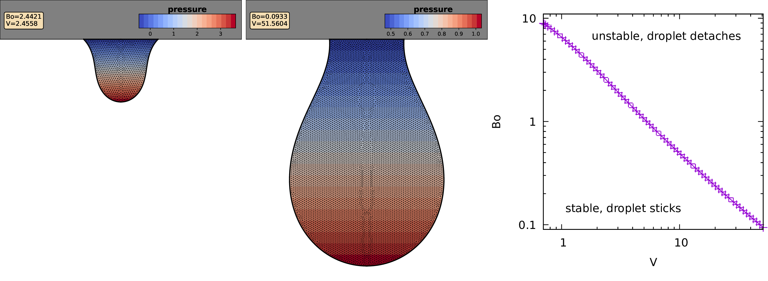
Fig. 10.3 Hanging droplets directly at the threshold to pinch-off due to gravity. Also the curve \(\operatorname{Bo}(V)\) is shown.