3.11.7. Bifurcation tracking
Finally, when a bifurcation point is a function of multiple parameters, one can jump on the bifurcation by adjusting one parameter and find the position of the bifurcation as a function of another parameter by arc length continuation. To that end, let us consider the Lorenz system (3.9) from Section 3.6.5. It is known that the Lorenz system has one trivial fixed point for \(\rho<1\), after which a supercritical pitchfork bifurcation can be found at \(\rho=1\), which eventually loses its stability in a subcritical Hopf bifurcation, whose location and presence are dependent on the parameters \(\sigma\) and \(\beta\). Beyond the Hopf bifurcation, chaotic behavior can be expected.
First of all, let us find the pitchfork bifurcation at \(\rho=1\) with pyoomph. To that end, the equations are loaded from the code from Section 3.6.5 and a problem class is defined where all three parameters can be adjusted at run time, i.e. are bound by define_global_parameter() and can hence be changed after the C code generation and can be used for arc length continuation and bifurcation tracking. We reuse the code of the file adaptive_lorenz_attractor.py from Section 3.6.5 here:
from adaptive_lorenz_attractor import * # import the Lorenz problem

# Simple Lorenz system where all parameters can be changed at runtime
class LorenzBifurcationProblem(Problem):
    def __init__(self):
        super(LorenzBifurcationProblem, self).__init__()
        self.rho=self.define_global_parameter(rho=0)
        self.sigma = self.define_global_parameter(sigma=0)
        self.beta = self.define_global_parameter(beta=0)

    def define_problem(self):
        ode=LorenzSystem(sigma=self.sigma,beta=self.beta,rho=self.rho)
        self.add_equations(ode@"lorenz")
First, find the pitchfork bifurcation as described in the previous section, including the analytically derived Hessian terms using setup_for_stability_analysis(). We must be somewhat close to the pitchfork bifurcation, so we start at \(\rho=0.5\), solve for the stationary solution and find the critical eigenvector as guess for \(\vec{v}_\text{g}\):
if __name__=="__main__":
    with LorenzBifurcationProblem() as problem:
        problem.quiet() # shut up and use the symbolical Hessian terms
        problem.setup_for_stability_analysis(analytic_hessian=True)

        # Start near the pitchfork at rho=1
        problem.rho.value=0.5
        problem.sigma.value=10
        problem.beta.value=8/3
        problem.solve(timestep=0.1) # Get the initial solution (trivial solution here)
        problem.solve()
        problem.solve_eigenproblem(0) # get an eigenvector as guess
Now we find the pitchfork and indeed confirm that it is at \(\rho=1\):
        # Find the pitchfork in terms of rho
        problem.activate_bifurcation_tracking(problem.rho,"pitchfork",eigenvector=problem.get_last_eigenvectors()[0])
        problem.solve()
        x,y,z=problem.get_ode("lorenz").get_value(["x","y","z"])
        print(f"Pitchfork starts at rho={problem.rho.value}, x,y,z={x,y,z}")
At a pitchfork bifurcation, we cannot easily continue in \(\rho\) since it is not clear which branch to take. Therefore, we obtain the critical eigenvector by get_last_eigenvectors(). As long as bifurcation tracking is active and it has been solved, it is not necessary (and not possible) to use solve_eigenproblem() for that. Instead, get_last_eigenvectors() gives the critical eigenvector at the bifurcation. We therefore first store this eigenvector and then deactivate the bifurcation tracking to be ready to solve the normal Lorenz system (i.e. without the augmentation for the bifurcation tracking):
        # this will be now the critical eigenvector at the bifurcation
        perturb=numpy.real(problem.get_last_eigenvectors()[0])
        # deactivate bifurcation tracking: Solve again the normal Lorenz system
        problem.deactivate_bifurcation_tracking()
To jump on the stable branch of the pitchfork bifurcation, we can add this eigenvector to the degrees of freedom using the perturb_dofs() method, increase \(\rho\) a bit beyond \(\rho>1\) and perform a few transient solves to move towards the stable branch, before the stationary solve jumps on it:
        problem.perturb_dofs(perturb) # Go in the direction of the critical eigenvector
        problem.rho.value+=0.1 # and go a bit higher with the rho value
        problem.solve(timestep=[0.1,1,2,None]) # do a few time steps and then a stationary solve (timestep=None)
        eigvals, eigvects=problem.solve_eigenproblem(0) # get the initial eigenvalues
Then, we gradually increase \(\rho\) by arc length continuation, solve for the eigenvalues and monitor whether the largest real part of the eigenvalues crosses zero:
        # Scan rho to the Hopf bifurcation
        ds=0.001
        while eigvals[0].real<-0.001:
            ds=problem.arclength_continuation(problem.rho,ds)
            x, y, z = problem.get_ode("lorenz").get_value(["x", "y", "z"])
            eigvals, eigvects = problem.solve_eigenproblem(0)
            print(f"On pitchfork branch rho={problem.rho.value}, x,y,z={x, y, z}, eigenvalue={eigvals[0]}")
The eigenvalue will have a non-zero imaginary value, which indicates a Hopf bifurcation. This means the critical eigenvalue will not be zero, but in fact a pair of imaginary values \(\pm i\omega\). For the same reason, the eigenvector \(\vec{v}\) will be complex (and a complex conjugate counter-pair), i.e. \(\vec{v}=\vec{\phi}+i\vec{\psi}\) with real valued \(\vec{\phi}\) and \(\vec{\psi}\). The bifurcation tracking of a Hopf bifurcation with respect to the parameter \(r\) (\(=\rho\) here) is internally again handled by augmenting the system as follows:
Besides the complex eigenvector \(\vec{v}=\vec{\phi}+i\vec{\psi}\), which can be obtained after bifurcation tracking by the two eigenvectors returned from get_last_eigenvectors(), one also gets the critical parameter, where the bifurcation happens, and the frequency \(\omega\), which can be obtained by the imaginary part of get_last_eigenvalues[0].
Now, this is utilized to find the critical \(\rho_\text{c}\) where the Hopf bifurcation is located:
        # Jump on the Hopf bifurcation
        problem.activate_bifurcation_tracking(problem.rho,"hopf",eigenvector=problem.get_last_eigenvectors()[0],omega=numpy.imag(problem.get_last_eigenvalues()[0]))
        problem.solve()
        x, y, z = problem.get_ode("lorenz").get_value(["x", "y", "z"])
        print(f"On Hopf branch rho={problem.rho.value}, x,y,z={x, y, z}, omega={numpy.imag(problem.get_last_eigenvalues()[0])}")
Since we do not deactivate_bifurcation_tracking(), it is still active. We can now perform an arc length continuation in another parameter, e.g. in \(\sigma\), to obtain the curve \(\rho_\text{c}(\sigma)\):
        # Go down with sigma but staying on the Hopf bifurcation (i.e. do not call deactivate_bifurcation_tracking)
        ds=-0.001
        while problem.sigma.value>2+problem.beta.value:
            ds=problem.arclength_continuation(problem.sigma,ds,max_ds=0.1)
            x, y, z = problem.get_ode("lorenz").get_value(["x", "y", "z"])
            print(f"On Hopf branch rho,sigma={problem.rho.value,problem.sigma.value}, x,y,z={x, y, z}, omega={numpy.imag(problem.get_last_eigenvalues()[0])}")
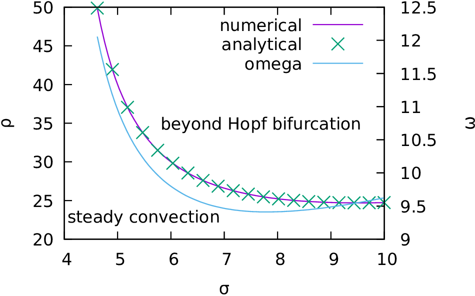
Fig. 3.14 Position of the Hopf bifurcation of the Lorenz system as a function of the parameters \(\rho\) and \(\sigma\) at \(\beta=8/3\). The analytical solution \(\rho_\text{c}=\sigma(\sigma+\beta+3)/(\sigma-\beta-1)\) agrees perfectly.
Thereby, one can directly generate phase diagrams as e.g. depicted in Fig. 3.14.
The very same methods also work for spatio-temporal differential equations. An example will be discussed in Section 5.6.