4.4.9. Adjusting a parameter so that a specified condition is met
In the following, we discuss a neat feature of fully-implicit methods: We have a problem that outputs an observable as function of a parameter. While such problems can be easily scanned to get a curve of the observable as function of the parameter (forward problem), we can also automatically adjust the parameter so that the observable attains some desired value (inverse problem).
4.4.9.1. Forward problem
Consider a rectangular cavity which is driven by tangential shear stress at the top boundary and no-slip on all other boundaries. The tangential shear stress at the top is given by a parameter \(T\) and we want to observe the induced velocity inside the cavity by the root-mean-square velocity
where \(A\) is the area of the cavity.
We can easily assemble such simple problems by using the predefined equations classes. We do not even have to define a specific Problem class, but instead assemble the problem directly:
from pyoomph import *
# Use the predefined NavierStokesEquations
from pyoomph.equations.navier_stokes import *

# Create a problem and define it in the run script directly instead of using inheritance
problem = Problem()
# The tangential traction at the top boundary is a parameter that we can adjust.
T = problem.define_global_parameter(T=0)

# Assemble the equations
eqs = NavierStokesEquations(mass_density=10, dynamic_viscosity=1)
eqs += MeshFileOutput()
eqs += NoSlipBC()@["left", "right", "bottom"]
eqs += (DirichletBC(velocity_y=0)+NeumannBC(velocity_x=T))@"top"
# Since we have no inflow/outflow, we need to fix the pressure, since p->p+const is a nullspace transformation.
eqs += AverageConstraint(pressure=0)

# To monitor the induced velocity, we define IntegralObservables
# First we calculate the integral of u^2 over the domain
# We also need the area of the domain, which is 1 in this case, but we calculate via integral of 1, which is relevant for more complicated domain
# Finally, U is given by sqrt(integral(u^2)/Area)
eqs += IntegralObservables(U_sqr=dot(var("velocity"), var("velocity")),
                           Area=1, U=lambda U_sqr, Area: square_root(U_sqr)/Area)

# Add mesh and equations
problem += RectangularQuadMesh(N=25, name="domain")
problem += eqs@'domain'

problem.solve()

# Scan to get a curve of U vs T
out_file = problem.create_text_file_output("U_vs_T.txt", header=["T", "U"])
for T_val in numpy.linspace(0, 100, 20, endpoint=True):
    problem.go_to_param(T=T_val)
    problem.output()
    U_val = problem.get_mesh("domain").evaluate_observable("U")
    out_file.add_row(T, U_val)
Main steps are again to define \(T\) as a global parameter, so that it can be scanned afterwards. Then, for the calculation of \(U\), we first have to split it into spatial integrals and finally express \(U\) in terms of these integrals.
This can all be achieved in a single IntegralObservables, where the last step in the calculation is obtained by a lambda using the correct parameter names to get the values from the spatial integrals. create_text_file_output() generates a file in the output directory, which is then written by scanning over \(T\) using go_to_param(). The results are plotted in Fig. 4.23.
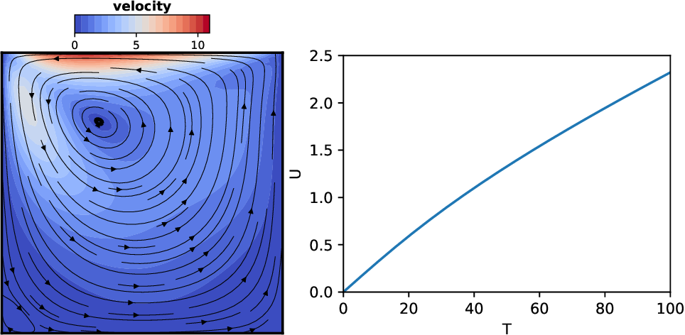
Fig. 4.23 (left) Velocity field inside the cavity for \(T=100\) . (right) RMS velocity \(U\) as function of \(T\)
4.4.9.2. Inverse problem
Consider you now want to adjust \(T\) so that the observable \(U\) attains some specific value \(U_\text{desired}\). Of course, you can look up the appropriate value of \(T\) from the graph in Fig. 4.23, but this requires to first solve the forward problem for an entire range of the parameter \(T\). A more sophisticated approach would be bisection in \(T\) until the condition \(U=U_\text{desired}\) is met.
However, fully-implicit solvers, as used in pyoomph, are capable of inverting the problem and of directly solving for \(T\) so that \(U=U_\text{desired}\) holds. Obviously, \(T\) is then not a free parameter anymore, but an unknown. Instead, we get \(U_\text{desired}\) as a parameter and the residual equation for \(T\) becomes
i.e. we adjust \(T\) so that we have the desired average velocity inside the cavity. To incorporate this equation into the problem, we first reformulate it to
\(R_T\) is now in a suitable residual formulation to be used directly in a weak form to find the value for \(T\).
So we first remove \(T\) as parameter and introduce \(U_\text{desired}\) instead. Then, \(T\) must be defined as an unknown:
#T = problem.define_global_parameter(T=0) # T is not a parameter anymore
Udesired=problem.define_global_parameter(Udesired=1) # Some value we want to reach for the rms-average velocity U=1
# T is now an unknown, adjusted to reach the desired U, so we define it as a dof instead of a parameter
# We must pass a reasonable initial condition for T to assist Newton's method for convergence
T,Ttest=problem.add_global_dof("T",initial_condition=10)
Since \(T\) is a single degree of freedom (i.e. not a field), we add it to the problem with add_global_dof(). It is important to provide a reasonable initial condition for \(T\), since Newton’s method can run into convergence issues otherwise.
Then, we add the equation for \(T\), which can be achieved by
# We want to adjust T, so that the residual R=integral(u^2) - Udesired^2 = 0
# So we just add the contribution integral(u^2) - Udesired^2 to the residual of T
eqs += WeakContribution(dot(var("velocity"), var("velocity")) - Udesired*Udesired, Ttest)
WeakContribution() is just an equation class which just adds a single contribution to the weak formulation. Here, just the spatial integral of \(\vec{u}^2 - U_\text{desired}^2\) over the domain to the residuals of \(T\).
There is one caveat for this particular equation, namely that it is quadratic in the velocity, i.e. \(\vec{u}^2\). By default, pyoomph starts with a zero velocity field, which then produces a zero Jacobian row in the first Newton iteration. So we first must find a reasonable guess for the velocity field without trying to adjust the unknown forcing \(T\). We therefore remove \(T\) from the degrees of freedom and solve for the velocity and pressure only:
# Newton's method cannot start with a zero velocity field, since u^2 will produce an empty Jacobian row.
# So we first have to solve the problem with T fixed, to get a reasonable starting guess for the velocity field
with problem.select_dofs() as dofs:
    # Remove T from the dofs, so that it is fixed in the first solve
    dofs.unselect("globals/T")
    # Solve the velocity and pressure for this fixed T
    problem.solve()
    # When leaving the 'with' block, T is an unknown again, and we can solve the full problem to adjust T to reach the desired U
select_dofs() should be used in a with statement. Different degrees of freedom can be then selected or unselected and all solve() commands within the with block are only performed on the selected (or not unselected) degrees of freedom. When leaving the with block, all degrees of freedom become active again, so that we can now solve for the full problem, including the adjustment of \(T\):
# Solve to adjust T to reach the desired U
problem.solve()

# Output results
print("To reach U=", Udesired.value, "we need T=", problem.get_ode("globals").get_value("T"))
print("U (calculated)=", problem.get_mesh("domain").evaluate_observable("U"))
Note that the definition of the unknown \(T\) via add_global_dof() above stores the unknown in an ODE called "globals". Therefore, we have to access the value of \(T\) using get_ode().
At this point, one could of course do a scan in \(U_\text{desired}\), but this would just yield the same plot as in the forward problem, just as the inverse function \(T(U_\text{desired})\).
Note
Finding a suitable initial condition for the parameter to be adjusted (\(T\) in the discussed inverse problem) is crucial. If it is hard to guess a reasonable initial value, one can replace \(T \leftarrow (1-\mu)T_0+\mu T\), where \(T_0\) is a constant (some initial guess) and \(\mu\) is a blending parameter. One can then start with \(\mu=0\) and gradually blend \(\mu\to 1\), e.g. via go_to_param(). However, to close the problem for \(\mu=0\), one has to add e.g. equation_contribution=(1-mu)*(var("T")-T0) to the add_global_dof definition of \(T\) and augment the WeakContribution with the factor \(\mu\), e.g. by using mu*Ttest as second argument. Thereby, for \(\mu=0\), the residual for \(T\) will be just \(T-T_0=0\), whereas for \(\mu=1\) one recovers the original form. In particular, also the issue with Newton’s method in the first step (due to the zero velocity field) is circumvented when starting with \(\mu<1\) (e.g. \(\mu=0\)).