7.3. Melting of an ice cylinder with natural convection
While it has been a lot of work to develop the rather simple example of a propagating ice front, we can now harvest the fruits of our labor by re-using these equations in higher dimensions and different geometries and add even more equations to the system.
As an example system, we consider the melting of an ice cylinder in a cylindrical bath of water. This has been investigated in Ref. [48], resulting in intriguing scalloped ice shapes due to a Kelvin-Helmholtz instability. We hence transfer the previous system into an axisymmetric variant, with an ice cylinder in the center and a liquid domain outside. In the liquid, also buoyancy driven flow will be relevant, where the density anomaly of water is important.
First of all, a mesh is required. We are lazy guys here: Although the geometry would allow us to build the elements by hand, we just use the GmshTemplate to construct a mesh via gmsh (cf. Section 4.3.4):
from temperature_conduction_propagation import * # Get some equations from the previous example
from pyoomph.equations.navier_stokes import * # We also need a Navier-Stokes equation

# We are lazy and use the Gmsh approach here instead of adding the elements by hand
class TwoDomainMeshAxi(GmshTemplate):
    def __init__(self,R1,R2,H,resolution):
        super(TwoDomainMeshAxi, self).__init__()
        self.R1,self.R2,self.H=R1,R2,H
        self.default_resolution=resolution

    def define_geometry(self):
        p00, p0H=self.point(0,0), self.point(0,self.H)
        pR10, pR1H=self.point(self.R1,0), self.point(self.R1,self.H)
        pR20, pR2H = self.point(self.R2, 0), self.point(self.R2, self.H)
        self.create_lines(pR10,"ice_bottom",p00,"axisymm",p0H,"ice_top",pR1H,"interface",pR10,"liquid_bottom",pR20,"liquid_side",pR2H,"liquid_top",pR1H)
        self.plane_surface("ice_bottom","axisymm","interface","ice_top",name="ice")
        self.plane_surface("liquid_bottom", "liquid_side", "interface", "liquid_top", name="liquid")
If you have read Section 4.3.4, nothing spectacular is happening here.
Next, we do not only solve thermal conduction, but also thermal convection in the liquid domain. We therefore must add the term \(\vec{u}\cdot\nabla T\) to our previously developed ThermalConductionEquation. This is most easily done by inheriting from the latter class:
# Augment the conduction equation by advection for the liquid phase
class ThermalAdvectionConductionEquation(ThermalConductionEquation):
    def __init__(self,k,rho,c_p,wind=var("velocity")):
        super(ThermalAdvectionConductionEquation, self).__init__(k=k,rho=rho,c_p=c_p)
        self.wind=wind

    def define_residuals(self):
        super(ThermalAdvectionConductionEquation, self).define_residuals() # define the conduction equation
        T,Ttest=var_and_test("T")
        self.add_residual(weak(self.rho*self.c_p*dot(self.wind,grad(T)),Ttest)) # Just add the advection term
Next, the problem will be defined. Although the problem is entirely different from the previous one, let us re-use it to copy the physical parameters as e.g. the conductivities and the latent heat:
# We inherit from the IceFrontProblem to take over the physical parameters. The problem will be quite different:
class IceConvectionProblem(IceFrontProblem):
    def __init__(self):
        super(IceConvectionProblem, self).__init__() # this will set all properties from the parent class
        self.L=4*centi*meter # L is now the cylinder height
        self.R1=1*centi*meter # radius of the ice cylinder
        self.R2=3*centi*meter # outer radius of the liquid cylinder

        self.T_ice=-1*celsius # initial ice cylinder temperature
        self.T_liq=6*celsius

        self.mu_liq=1*milli*pascal*second
        # Water density for buoyancy calculations
        Trel = (var("T") - self.T_eq) / kelvin # bind the relative temperature (measured in Kelvin)
        # Fit for the density anomaly
        self.rho_grav = (0.999849 + 5.77393e-05 * Trel - 7.18258e-06 * Trel ** 2) * gram / (centi * meter )** 3
        self.gravity=9.81*meter/second**2 * vector(0,-1) # gravity direction and strength

        self.resolution=0.05 # mesh resolution
Besides copying the parameters from the previous problem, where L is now used for the height of the cylinder, we need two radii, the viscosity of water and a fit for the density anomaly as a function of the temperature. Therefore, we normalize the actual relative temperature \(T-T_\text{eq}\) by the unit \(\:\mathrm{K}\) and plug this into a fit for the liquid water mass density between \(0\:\mathrm{^\circ C}\) and \(20\:\mathrm{^\circ C}\).
The define_problem() method starts again by adding the mesh, but this time we have a two-dimensional mesh and switch to an "axisymmetric" coordinate system. The scales are set as in the previous problem, but we require additional scales for the "velocity" and "pressure" fields:
    def define_problem(self):
        # Two-dimensional mesh
        self.add_mesh(TwoDomainMeshAxi(self.R1,self.R2,self.L,self.resolution))
        self.set_coordinate_system("axisymmetric") # axisymmetric coordinate system

        # Similar to the previous problem, scales for nondimensionalization
        self.set_scaling(spatial=self.R1,temporal=1*second)
        self.set_scaling(T=kelvin)
        self.set_scaling(thermal_equation=scale_factor("T") * self.k_ice / scale_factor("spatial") ** 2)
        self.set_scaling(velocity=scale_factor("spatial")/scale_factor("temporal"))
        self.set_scaling(pressure=self.mu_liq*scale_factor("velocity")/scale_factor("spatial"))
Next, the ice equations are assembled. They are essentially the same, except that we must add a few extra DirichletBC terms to fix the mesh at the top and bottom boundary. Furthermore, there is no DirichletBC for the temperature here, except the equilibrium temperature at the "interface". The ice cylinder will just warm up to \(0\:\mathrm{^\circ C}\) over the course of the simulation:
        self.add_mesh(TwoDomainMeshAxi(self.R1,self.R2,self.L,self.resolution))
        self.set_coordinate_system("axisymmetric") # axisymmetric coordinate system

        # Similar to the previous problem, scales for nondimensionalization
        self.set_scaling(spatial=self.R1,temporal=1*second)
        self.set_scaling(T=kelvin)
        self.set_scaling(thermal_equation=scale_factor("T") * self.k_ice / scale_factor("spatial") ** 2)
        self.set_scaling(velocity=scale_factor("spatial")/scale_factor("temporal"))
        self.set_scaling(pressure=self.mu_liq*scale_factor("velocity")/scale_factor("spatial"))

        # Equations for the ice domain
        ice_eqs=MeshFileOutput() # Output
        ice_eqs+=ThermalConductionEquation(self.k_ice,self.rho_ice,self.cp_ice) # thermal conduction
        ice_eqs +=InitialCondition(T=self.T_ice) # initially at ice temperature
        ice_eqs+=PseudoElasticMesh() # Mesh motion
        ice_eqs+=DirichletBC(mesh_x=0)@"axisymm" # fix mesh at axis of symmetry
        ice_eqs += DirichletBC(mesh_y=0) @ "ice_bottom" # and at the bottom
        ice_eqs += DirichletBC(mesh_y=self.L) @ "ice_top" # and the top
        ice_eqs += DirichletBC(T=self.T_eq)@"interface" # melting temperature at interface
The liquid equations are analogous, except that we use our new class ThermalAdvectionConductionEquation for the convection term and also add a NavierStokesEquations for the flow, together with no-slip boundary conditions at all interfaces. In reality, the density difference between ice and liquid would give rise to a non-zero normal velocity, when ice melts or solidifies, but this is not considered here, since this contribution is tiny. One could enforce this velocity jump via a Lagrange multiplier, but then, we also would allow for outflow somewhere in the domain to compensate for the gained/lost volume, i.e. to be able to satisfy the continuity equation. Since we do not allow any outflow, one pressure degree of freedom must also be fixed to remove the nullspace of the pressure (cf. Section 4.4.4):
        # Equations for the liquid domain
        liq_eqs=MeshFileOutput() # output
        liq_eqs+=ThermalAdvectionConductionEquation(self.k_liq,self.rho_liq,self.cp_liq) # thermal conduction + advection
        # Navier-Stokes including Boussinesq-like gravity term
        liq_eqs+=NavierStokesEquations(mass_density=self.rho_liq,dynamic_viscosity=self.mu_liq,bulkforce=self.gravity*self.rho_grav)
        liq_eqs+=InitialCondition(T=self.T_liq) # Liquid temperature as initial condition
        liq_eqs+=PseudoElasticMesh() # Mesh motion
        liq_eqs+=DirichletBC(mesh_y=0,velocity_x=0,velocity_y=0)@"liquid_bottom" # no-slip and fixed mesh at all boundaries
        liq_eqs += DirichletBC(mesh_y=self.L,velocity_x=0,velocity_y=0) @ "liquid_top"
        liq_eqs += DirichletBC(mesh_x=self.R2,T=self.T_liq,velocity_x=0,velocity_y=0)@"liquid_side"
        liq_eqs+=DirichletBC(T=self.T_eq,velocity_x=0,velocity_y=0)@"interface" # here the mesh is not fixed, but the temperature is
        liq_eqs += DirichletBC(pressure=0) @ "liquid_top/liquid_side" # For pure DirichletBCs, we must fix one pressure degree
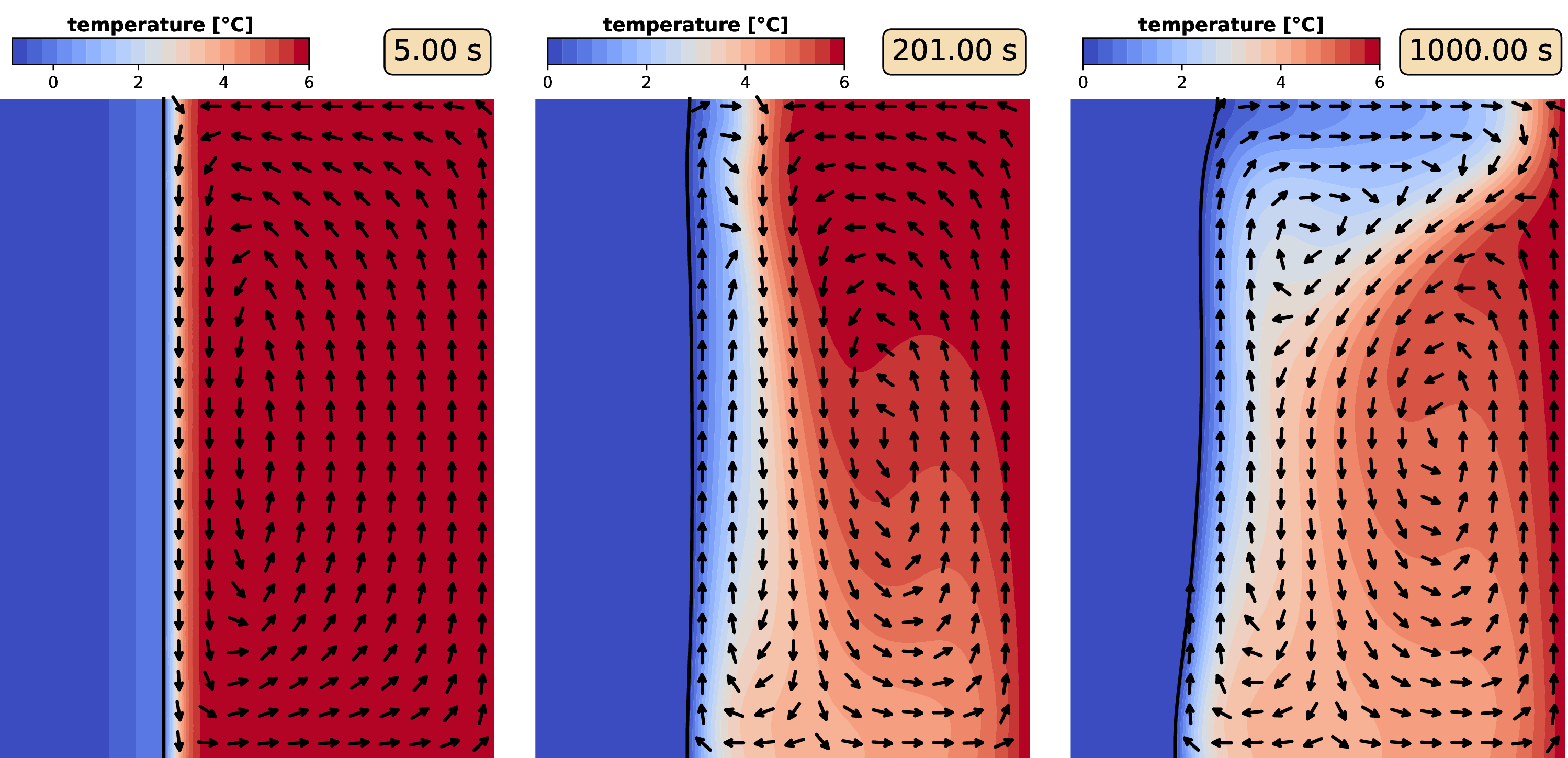
Fig. 7.3 Dynamics of an ice cylinder melting in a liquid bath along with natural convection due to the density anomaly.
Optionally, we can simplify the problem: Since the front will mainly move in radial direction, we can remove all degrees of freedom associated with the \(y\)-coordinate of the mesh:
        # Since we know that the mesh mainly moves in y-direction, we can speed up the calculation by removing the motion in y-direction
        ice_eqs += DirichletBC(mesh_y=True)
        liq_eqs += DirichletBC(mesh_y=True)

        # Reduce the bulk positions to be first-order, but allow the interface nodes to have a curvature per element
        ice_eqs += ConstrainPositionsToC1Space()+UnconstrainPositionsFromC1Space()@"interface"
        liq_eqs += ConstrainPositionsToC1Space()+UnconstrainPositionsFromC1Space()@"interface"
Thereby, we have fewer degrees of freedom in our system and the computation will speed up.
Also, note the additional feature we are using here, namely the classes ConstrainPositionsToC1Space and UnconstrainPositionsFromC1Space. The former enforces that the moving mesh is solved on first order elements everywhere inside both domains, i.e. while still having 9 nodes per second-order quadrilateral elements, the mesh dynamics is only solved on the 4 vertex nodes ("C1" space). However, at the interface, we want to include the possibility of having a curved boundary. Therefore, it is unconstrained there, i.e. the free surface can still deform as second-order elements.
In principle, we could have done the same with the temperature field using the classes ConstrainFieldsToC1Space and UnconstrainFieldsFromC1Space, respectively. However, since we pin the temperature at the interface, it would be equivalent to entirely degrade the temperature field to "C1", since the unconstraining would only act directly on the interface to resolve tangential gradients. Nevertheless, since the mesh motion usually does not matter for the physics, the reduction in the moving mesh order reduces the degrees of freedom and the computation time by about 25% without any notable downsides regarding the physics.
Finally, the interface equations are added as in the previous example and all equations are added to the problem:
        # Interface: Connect the mesh position and impose the front motion
        interf_eqs=ConnectMeshAtInterface()
        interf_eqs+=IceFrontSpeed(self.latent_heat)

        # Add it to the ice side of the interface
        ice_eqs+=interf_eqs@"interface"

        # and add all equations to the problem
        self.add_equations(ice_eqs@"ice"+liq_eqs@"liquid")
The code for execution is trivial:
if __name__=="__main__":
    with IceConvectionProblem() as problem:
        problem.run(400*second,outstep=True,startstep=1*second,maxstep=20*second,temporal_error=1)
The corresponding results are shown in Fig. 7.3. Obviously, the interface indeed does not recede in a straight manner, but is deformed due to the natural convection. Based on the results, one can obviously simplify the problem by neglecting the ice phase, since it becomes isothermal at \(T_\text{eq}=0\) very quickly. This would involve the modification of the IceFrontSpeed, but since this chapter is on multi-domain problems, it will not be addressed here.