8.6. Evaporation from a capillary & the geometric conservation law (GCL)

We want to apply the multi-component flow equations to the evaporation of a mixture from a capillary tube, analogously to what has been done in Ref. [41]. As in this reference, we consider the tube, filled with a mixture of glycerol and water, as a 1d system. At the bottom of the tube, water is evaporating, leaving the non-volatile glycerol behind. This implies that the total mass of glycerol inside the liquid must be conserved.

However, for simple ALE methods which just use partial_t(...,ALE=True), i.e. the ALE-corrected time derivative partial_t() (see Section 6.3), we will see that it does not perfectly conserve the total mass of glycerol. Instead, we get a time-step-dependent conservation, which is a typical result when using ALE without respecting the geometric conservation law.

If we want to have conservation up to machine-precision, float truncation and the Newton solver threshold, we must ensure that Reynolds transport theorem is satisfied. In the present case, we have to e.g. solve the advection-diffusion equation for the glycerol mass fraction \(w_\mathrm{g}\) in the liquid phase. For this binary mixture, the equation (8.1) reads

(8.6)\[\begin{aligned} \rho\left(\partial_t w_\mathrm{g}+\vec{u}\cdot\nabla w_\mathrm{g}\right)=\nabla\cdot\left(\rho D_{\mathrm{gw}} \nabla w_\mathrm{g}\right) \end{aligned}\]

For a test function \(\phi\), the weak form of this equation reads

(8.7)\[\begin{aligned} \left(\rho\left(\partial_t w_\mathrm{g}+\vec{u}\cdot\nabla w_\mathrm{g}\right),\phi\right) + \left(\rho D_{\mathrm{gw}} \nabla w_\mathrm{g},\nabla \phi\right)=\left\langle\rho D_{\mathrm{gw}} \nabla w_\mathrm{g},\mathbf{n} \phi\right\rangle \end{aligned}\]

This is how pyoomph implements the equation by default, where the time derivative considers the ALE correction on moving meshes. However, as shown below, this does not perfectly conserve the total mass of glycerol in the capillary.

Alternatively, we can use the continuity equation of (8.1) to rewrite (8.6) in a conservative form as

(8.8)\[\begin{aligned} \partial_t (\rho w_\mathrm{g})+\nabla\cdot(\rho\vec{u} w_\mathrm{g})=\nabla\cdot\left(\rho D_{\mathrm{gw}} \nabla w_\mathrm{g}\right) \end{aligned}\]

For the corresponding weak form, we want to make sure that the change of the volume of each element is taken into account, i.e. the time derivative is applied on the entire integral in the weak formulation, considering the changing integration domain.

(8.9)\[\begin{aligned} \frac{\mathrm{d}}{\mathrm{d}t} \left(\rho w_\mathrm{g},\phi\right) -\left(\rho (\vec{u}-\dot{\vec{x}})w_\mathrm{g},\nabla \phi\right) + \left(\rho D_{\mathrm{gw}} \nabla w_\mathrm{g},\nabla \phi\right)=\left\langle\rho D_{\mathrm{gw}} \nabla w_\mathrm{g} - \rho (\vec{u}-\dot{\vec{x}})w_\mathrm{g},\mathbf{n} \phi\right\rangle \end{aligned}\]

The time-derivative acts now on the entire integral and the advection term was integrated by parts, giving also rise to a boundary term, i.e. Neumann conditions are now not just the diffusive fluxes as before, but also comprise advective fluxes. The ALE correction is now incorporated directly in the advective term with the mesh velocity \(\dot{\vec{x}}\). In pyoomph, the time derivative of a weak form integral can be implemented using the time_derivative_of_integral() function, e.g. time_derivative_of_integral(weak(rho*w_g,phi)).

On a continuous level, both approaches are equivalent, but on a discrete level, the conservative form is more accurate in terms of conservation.

However, on the discrete level, there is another aspect to consider: the geometric conservation law (GCL). In order to fulfill Reynolds transport theorem, the discrete mesh velocity must be consistent with the discrete time derivative of the element volume. This is not automatically guaranteed in ALE methods. For first order time stepping with "BDF1", the GCL is automatically satisfied, but for higher order time stepping, it is not.

Note

At the moment, pyoomph does not fully handle the GCL for higher order time stepping, but the results are still much better in conservative form as seen below. The flag is still called GCL in the CompositionFlowEquations class, since it might be updated in future.

The multi-component flow equations can activate the conservative form by setting GCL=True in the CompositionFlowEquations. This also augments the Navier-Stokes equation and adjusts e.g. the evaporation boundary conditions to account for the changed Neumann terms. Custom Neumann conditions, e.g. a diffusive influx on a boundary, must be adjusted accordingly.

Let us now assess the conservation of the total mass of glycerol in the capillary tube. The code is just a quite simple 1d problem, i.e. the problem is initialized as follows:

from pyoomph import *
from pyoomph.equations.multi_component import *
from pyoomph.equations.ALE import *
from pyoomph.materials import *
from pyoomph.materials.mass_transfer import *
import pyoomph.materials.default_materials 

class CapillaryEvaporationProblem(Problem):
    def __init__(self):
        super().__init__()
        # Filled height in the capillary
        self.L=20*milli*meter
        # Capillary radius
        self.R=0.5*milli*meter        
        # Temperature of the system
        self.temperature=20*celsius
        # Initial Liquid mixture composition (glycerol/water)
        self.mixture=Mixture(20*percent*get_pure_liquid("glycerol")+get_pure_liquid("water"))
        # Gas phase composition (air with 20% relative humidity)
        self.gas=Mixture(get_pure_gas("air")+50*percent*get_pure_gas("water"),quantity="relative_humidity",temperature=20*celsius)
        # Gravity and ambient pressure
        self.g=9.81*meter/second**2
        self.ambient_pressure=1*atm
        # Whether we use the conservative form (better GCL agreement) or not
        self.use_GCL=True

For the define_problem() method we must setup a 1d moving mesh with multi-component flow equations. The "left" boundary represents the bottom of the capillary, the "right" boundary represents the top. We also have to extract a reasonable time and velocity scale, which can be inferred from the water evaporation rate. For the evaporation rate, we need the far field water mass concentration, which we extract from the gas mixture provided.

    def define_problem(self):
        self+=LineMesh(size=self.L,N=1000)
        
        # Get the interface properties
        interf=self.mixture | self.gas
        c_water=self.mixture.get_vapor_mass_concentration("water",at_mixture_composition=False)
        # get the water mole fraction in the gas phase, calculate the relative humidity and use it to calculate the far-field water vapor concentration
        xWater=self.gas.evaluate_at_condition(self.gas.get_mole_fraction_field("water"),"IC", temperature=self.temperature,pressure=self.ambient_pressure)
        psat=self.mixture.evaluate_at_condition(self.mixture.get_vapor_pressure_for("water",pure=True),temperature=self.temperature)
        xSat=psat/self.ambient_pressure
        RH=xWater/xSat        
        # and use it to calulate the far-field water vapor concentration
        c_infty=self.mixture.get_vapor_mass_concentration("water",relative_humidity_for_far_field=RH,temperature=self.temperature)
        # Get the diffusion coefficient of water in air at the given temperature
        D_vap=self.gas.get_diffusion_coefficient("water")(temperature=self.temperature)
        # And the evaporation rate        
        j_water=4*D_vap*(c_water-c_infty)/self.R        
        
        # The evaporation rate at the initial condition is used to define the velocity scale for the problem
        j_water0=self.mixture.evaluate_at_condition(j_water,"IC",temperature=self.temperature)
        rho0=self.mixture.evaluate_at_condition(self.mixture.mass_density, "IC", temperature=self.temperature)
        Uscale=j_water0/rho0
       
        # Set reasonable scaling for the problem
        self.set_scaling(spatial=self.L,velocity=Uscale,pressure=rho0*self.g*self.L)
        self.define_named_var(temperature=self.temperature)
        self.mixture.set_reference_scaling_to_problem(self,temperature=self.temperature)
        
        # Flow and composition in the bulk, optionally using the GCL
        eqs=CompositionFlowEquations(self.mixture,gravity=self.g*vector(-1),GCL=self.use_GCL)
        # output and a fixed position at the left side (bottom of the capillary) where the liquid evaporates
        eqs+=LaplaceSmoothedMesh()
        eqs+=TextFileOutput()
        eqs+=DirichletBC(mesh_x=0)@"left" # Open part of the capillary, evaporating from here
        
        # Use a prescribed mass transfer model to impose the evaporation rate at the interface
        mdl=interf.set_mass_transfer_model(PrescribedMassTransfer(water=j_water))
        mdl.projection_space="C2" # Project the evaporation rate onto a continuous quadratic space (here, the space does not matter)
        eqs+=MultiComponentNavierStokesInterface(interf,static=True)@"left"
        
        # The right side of the capillary is allowed to move, but no evaporation is allowed there
        interf_no_evap=self.mixture | self.gas
        interf_no_evap.set_mass_transfer_model(None)
        eqs+=MultiComponentNavierStokesInterface(interf_no_evap)@"right"
        
        # Get the total mass of glycerol
        eqs+=IntegralObservables(M_glycerol=var("massfrac_glycerol")*self.mixture.mass_density*pi*self.R**2)
        eqs+=IntegralObservableOutput("mass_evolution")
        # Get the filled height and it's velocity
        eqs+=IntegralObservables(y=self.L-var("mesh_x"),u=-mesh_velocity()[0])@"right"
        eqs+=IntegralObservableOutput("top_interface")@"right"
        
        # Refine the region near the evaporating interface to better resolve the gradients in the solution
        eqs+=RefineToLevel(4)@"left"
        
        self+=eqs@"domain"

There are two MultiComponentNavierStokesInterface objects, one at the bottom ("left") and one at the top ("right"). The bottom interface is where the evaporation takes place, and we prescribe the evaporation rate using a PrescribedMassTransfer model. This interface is static, i.e. fixed in position. The kinematic boundary condition therefore acts on the velocity, not on the mesh motion. The top interface is allowed to move, but no evaporation is allowed there. Here, the kinematic boundary condition acts on the mesh motion. Note also that we pass GCL=self.use_GCL to the CompositionFlowEquations object, which will ensure that the conservative form of the equations is used when self.use_GCL=True.

To run the simulation, we again use dynamic time stepping, which perfectly adapts to the logarithmic plots in Fig. 8.3:

if __name__=="__main__":
    with CapillaryEvaporationProblem() as problem:
        problem.DTSF_max_increase_factor=1.25
        problem.DTSF_min_decrease_factor=0.75
        problem.run(48*hour,outstep=True,startstep=0.001*second,temporal_error=1)

The results in Fig. 8.3 show the concentration of glycerol in the capillary at different times, the velocity of the top interface, receding due to evaporation at the bottom, and the total mass of glycerol in the capillary. The total mass of glycerol is not perfectly conserved when using ALE with GCL=False, but is conserved nicely when using the GCL.

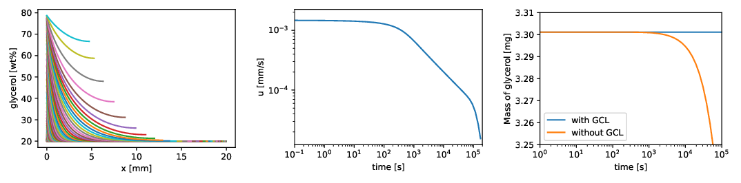
Fig. 8.3 Evaporation of a glycerol-water mixture from a capillary tube. (left) the concentration of glycerol in the capillary at different times. (middle) the velocity of the top interface, receding due to evaporation at the bottom. (right) the total mass of glycerol in the capillary, which is not perfectly conserved when using ALE without GCL, but is conserved nicely when using the GCL.

Download this example

Download all examples