6.6. Remeshing by reconstruction, gmsh size fields & zeta coordinates
As explained in Section 6.4, remeshing can be treated quite automatically. However, sometimes, it is required to have more control over the local mesh size in this procedure. Also, sometimes you know the exact location of some boundaries, e.g. solid walls will always stay in place and an axis of symmetry will always be located at \(r=0\).
Both of these aspects are tackled with the class RemeshableGmshTemplate2d. This class behaves like a normal GmshTemplate, but its define_geometry() method will be called again for each remeshing event. Of course, the free surface will have moved by then, so we require two ingredients to realize this approach:
Within the method
define_geometry(), we must be able to find out whether we are constructing the initial mesh or whether we are remeshing. This can be checked with the methodis_first_time(). For the initial mesh, this yieldsTrue, i.e. we can mesh the initial shape of the free surface. If it isFalse, we are remeshing, so we must reconstruct the current shape of each free surface.In the latter case, we must find the points defining the current shape, so that a new boundary of the same shape can be created, typically a spline. The points of the current boundary, i.e. the one we want to reconstruct, are accessible via the method
get_boundary_coordinates().
In the following, we will examplify this approach by the well-known Rayleigh-Plateau instability of a liquid cylinder.
from pyoomph import *
# Using the predefined Navier-Stokes and ALE equations from pyoomph
from pyoomph.equations.navier_stokes import *
from pyoomph.equations.ALE import *
# We require the remeshing utities from pyoomph
from pyoomph.meshes.remesher import *
# And the interface zeta coordinate utilities to get smooth interpolation of the interface upon remeshing
from pyoomph.meshes.zeta import *


class DomainMeshAxi(RemeshableGmshTemplate2d):
    def define_geometry(self):
        self.mesh_mode="tris"

        # Setting some GMSH global options
        pr=cast(RayleighPlateauProblem, self.get_problem())
        # Never make a finer mesh than the minimum radius threshold would allow
        self.gmsh_options["Mesh.MeshSizeMin"]=pr.epsilon/pr.min_elements_per_radius
        # Make sure that we cannot go coarser than the maximum elements per radius
        self.gmsh_options["Mesh.MeshSizeMax"]=1.0/pr.max_elements_per_radius
        # Make sure that we have enough elements to resolve the curvature of the interface
        self.gmsh_options["Mesh.MeshSizeFromCurvature"]=8*pr.min_elements_per_radius
We inherit from the class RemeshableGmshTemplate2d and override the method define_geometry() as usual.
However, we now give additional mesh size control to Gmsh by setting several values via the gmsh_options. In particular, we set a minimum mesh size depending on the desired resolution and the minimum radius of the problem class (specified later therein), a maximum mesh size and enhance strongly curved parts of the interface by finer resolution.
All available Gmsh options can be found in the documentation .
Then, we perform the steps mentioned at the top, i.e. create an initial mesh or reconstruct the interface by a spline, depending on whether is_first_time() is True or False:
        # The end points on the axis are always the same
        p00,p0H=self.point(0,0),self.point(0,pr.L)

        if self.is_first_time():
            # We just create a rectangle as initial mesh and perturb it afterwards
            pR0,pRH=self.point(1,0),self.point(1,pr.L)
            interface=self.line(pR0,pRH,name="interface")
        else:
            # Remeshing: We need the current interface shape
            interface_segments=self.get_boundary_coordinates("liquid/interface",sort_along_axis="y+")
            # There is only one segment in the interface, but we still need to create a list of Gmsh points
            pts=[self.point(x,y) for x,y in interface_segments[0]]
            # We create a spline through the points to define the interface
            interface=self.spline(pts,name="interface")
            # the end points of the interface are just used for the top and bottom corners
            pR0,pRH=pts[0],pts[-1]

        # Common part: Axis of symmetry and the top and bottom lines and the surface
        axis=self.create_lines(pR0,"bottom",p00,"axisymm",p0H,"top",pRH)[1]
        self.plane_surface("bottom","axisymm", "top","interface",name="liquid")
The axis of symmetry is always the same in this case, so we can always create these points. We do not set any mesh size here, since it will be treated in another way soon. For the initial mesh, we just make a box, for the remeshing steps, we get the coordinates of the current interface by get_boundary_coordinates(). This results in a list of boundary segments. Here, however, we only have a single segment, since the interface will always be a single connected curve. We can sort the points along the boundary automatically with the argument sort_along_axis="y+". Even in case of overhangs, the order is still following the curve, i.e. this sorting is performed based on the end points only. We then construct the points, pass them to a spline and extract the start and end points of the surface at the bottom and top, before meshing the domain as usual in both scenarios, the initial mesh and each reconstructed mesh.
For the mesh size, we use gmsh’s mesh size fields, which can be added with add_mesh_size_field() method:
        # Now define mesh size fields of gmsh (see https://gmsh.info/doc/texinfo/#Gmsh-mesh-size-fields)

        # First, calculate the distance from the interface to the axis of symmetry.
        # This is just the radius, so we just use a "MathEval" with the x-coordinate.
        # We divide by the minimum elements per radius to get the desired mesh size.
        dist_interf_to_axis=self.add_mesh_size_field("MathEval",F="x/"+str(pr.min_elements_per_radius))
        # However, this resolution is only meant for the interface, so we restrict it with a "Restrict" field to the interface curve
        restr_interf=self.add_mesh_size_field("Restrict",InField=dist_interf_to_axis,CurvesList=[interface])
        # For the resolution on the axis, we need to calculate the distance from the axis to the interface.
        # This is done with a "Distance" field, but it is important to increase the "Sampling" parameter here
        axis_to_inter=self.add_mesh_size_field("Distance",CurvesList=[interface],Sampling=1000)
        # Convert the distance to a mesh size using "MathEval".
        # We can access the value of the distance field with "F<field_id>", where <field_id> is the id of the distance field.
        axis_to_inter_size=self.add_mesh_size_field("MathEval",F="F"+str(axis_to_inter)+"/"+str(pr.min_elements_per_radius*0.75))
        # Again, we restrict this mesh size to the axis of symmetry with a "Restrict" field
        restr_axis=self.add_mesh_size_field("Restrict",InField=axis_to_inter_size,CurvesList=[axis])
        # Now we just take the minimum of the two restricted mesh size fields to get the final mesh size field
        combined=self.add_mesh_size_field("Min",FieldsList=[restr_interf,restr_axis])
        # And tell gmsh to use this one
        self.set_mesh_size_background_field(combined)
If the filament gets thin, we must take a finer resolution. This can be realized by setting the mesh size at the "interface" to the value of the radial coordinate. Gmsh offers a "MathEval" field, which can evaluate any expressions involving e.g. the coordinates "x", "y" and "z". Here, we scale it by the minimum desired elements per radius. The resulting expression has to be passed via the F property of the "MathEval" field, which is just passed as kwargs to the add_mesh_size_field() call. This field alone would refine the mesh near the axis of symmetry, since the radial coordinate is tiny there. Therefore, we must use a "Restrict" to confine this size field to the interface. The same can be done with the axis of symmetry, which should be meshed the finer the closer the interface approaches. We cannot get away with a "MathEval" here, but we use a "Distance" field first to calculate the distance to the interface. It is key to increase the "Sampling" here to get an accurate distance. This is then passed again to a "MathEval" to calculate the mesh resolution from the distance and finally restricted to the axis itself. Eventually, both restricted fields are combined by the "Min" field, which is then set as mesh size field via set_mesh_size_background_field(). Gmsh will then evaluate the mesh sizes, which only results in reasonable values at the interface and the axis (due to the restricting). In the bulk, by default, Gmsh interpolates the mesh sizes from the boundaries.
The problem definition starts as usual:
class RayleighPlateauProblem(Problem):
    def __init__(self):
        super().__init__()
        self.L=4.0 # Length of the domain
        self.Oh=0.07 # Ohnesorge number
        self.k=pi/4 # Wavenumber of the perturbation
        self.a=0.1 # Amplitude of the perturbation
        self.min_elements_per_radius=2 # Resolution of the mesh, typical elements per radius (higher means finer mesh)
        self.max_elements_per_radius=4 # Maximum elements per radius (higher means finer mesh)
        self.epsilon=0.0004 # Minimum radius threshold for stopping the simulation

    def define_problem(self):
        self.add_mesh(DomainMeshAxi())
        self.set_coordinate_system("axisymmetric")

        # Equations
        eqs=NavierStokesEquations(mass_density=1,dynamic_viscosity=self.Oh)
        eqs+=HyperelasticSmoothedMesh()
        eqs+=MeshFileOutput()
        # We still must tell pyoomph that it should remesh when necessary
        eqs+=RemeshWhen(RemeshingOptions())

        # Initial perturbation
        X,Y=var(["lagrangian_x","lagrangian_y"])
        eqs+=InitialCondition(mesh_x = X*(1+self.a*cos(self.k*Y)))

        # Boundary conditions
        eqs+=AxisymmetryBC()@"axisymm"
        eqs+=DirichletBC(mesh_y=True)@["top","bottom"]
        eqs+=DirichletBC(velocity_y=0)@["bottom","top"]
        eqs+=NavierStokesFreeSurface(surface_tension=1)@"interface"

        # Monitor the minimum radius and its position along the interface
        eqs+=ExtremumObservables(min_r=var("mesh_x"))@"interface"
The only novel part are the ExtremumObservables, which will be used to evaluate the minimum radius and its position soon. We define the minimum (and maximum) radius min_r by the minimum (and maximum) value of var("mesh_x").
One imporant aspect about remeshing is the accurate interpolation from the old to the reconstructed mesh. pyoomph does this automatically, but for interfaces, it can be improved. Normally, pyoomph interpolates values on interfaces at a point by the two nearest neighboring nodes of the old mesh. This, however, does not always give the best results. Instead, a unique mapping from the new to the old interface is relevant, for which oomph-lib has introduced so-called zeta coordinates. For an interface, we need a single value as parametrization, but the parametrization of the old and new interface must result in the same position. For the axis of symmetry, we can therefore set \(\zeta=y\), for the top and bottom, we can use \(\zeta=x\). For the curved interface, we might expect overhangs, meaning that e.g. \(\zeta=y\) might not be a unique mapping. The (normalized) arclength, however, is always a good \(\zeta\) parametrization, provided it starts at the same point in both the old and the reconstructed mesh. If \(\zeta\) is defined on a boundaries, the interpolation from the old to the new boundary is then performed via the \(\zeta\) coordinate, which is considerably more accurate and less error-prone than the default linear interpolation between the nearest neighbors. To set up the \(\zeta\) coordinates, we use the classes from pyoomph.meshes.zeta:
        # This improves the interpolation at interfaces upon remeshing
        eqs+=AssignZetaCoordinatesByEulerianCoordinate("x")@"bottom"
        eqs+=AssignZetaCoordinatesByEulerianCoordinate("x")@"top"
        eqs+=AssignZetaCoordinatesByEulerianCoordinate("y")@"axisymm"
        eqs+=AssignZetaCoordinatesByArclength(sort_along_axis="y+")@"interface"

        self.add_equations(eqs@"liquid")
These lines realize our thoughts above, i.e. all boundaries now have a \(\zeta\) coordinates, which coindice with the relevant Cartesian coordinate for "bottom", "top" and "axisymm" via the AssignZetaCoordinatesByEulerianCoordinate and follows the normalized arclength on the "interface". In the AssignZetaCoordinatesByArclength, we have opted to start with \(\zeta=0\) at the bottom by passing sort_along_axis="y+", which uniquely and consistently defines \(\zeta\) also on this boundary.
To run the simulation, we want to make sure that time stepping gets smaller when the minimum radius decreases. While pyoomph’s adaptive time stepping will also take care of this in a rudimentary way, a manual adjustment can be beneficial, in particular when one is interested in a rather equidistant logarithmic plot as shown below. The rest of the problem definition script therefore reads as follows:
    def get_minimum_radius_and_position(self):
        # Obtain the minimum radius and its position along the interface
        # evaluate_minimum with return_x=True returns a tuple of (min_value, (x,y)), so we unpack it accordingly
        min_r,min_z=self.get_mesh("liquid/interface").evaluate_minimum("min_r",return_x=True)[1]
        return min_r,min_z

    def minimum_radius_dependent_run(self,dt_factor=0.1,maxstep=0.1):
        # This is a generator function that yields the current time and adjusts the time step based on the minimum radius
        while True:
            r_min,_=self.get_minimum_radius_and_position()
            if r_min<self.epsilon:
                return # Stop the run if the minimum radius is below the threshold

            dt=dt_factor*r_min # Time step is proportional to the minimum radius

            if dt>maxstep:
                dt=maxstep # Limit the maximum time step to avoid too large steps

            # Run a simulation over the time interval [t, t+dt] and yield the current time after each step
            # We might take multiple steps within this interval if necessary, but we only yield after the full interval
            self.run(self.get_current_time()+dt,outstep=False,maxstep=dt,temporal_error=1)
            yield problem.get_current_time()
First we introduce a getter function to obtain the minimum radius and its axial position. We can use the method evaluate_minimum() to evalute the minimum of the the expression defined by the ExtremumObservables above, here min_r=var("mesh_x"). Passing return_x=True will also return the location of the minimum as second result, which we return by the first method above. Of course, there is also an analogous function function evaluate_maximum(), but his is less interesting here.
The second method above just runs the simulation over small intervals in time, where the size of this interval is chosen based on the minimum radius. It is written as generator so that it can be used in the main script as follows:
if __name__=="__main__":
    with RayleighPlateauProblem() as problem:
        # Control the time step adaptation factors
        problem.DTSF_max_increase_factor=1.25 # increase dt by 25% for successful steps
        problem.DTSF_min_decrease_factor=0.75 # decrease dt by 25% for failed steps

        problem.initialise()
        # Monitor the minimum radius and its position along the interface and write to a text file
        minimum_out=problem.create_text_file_output("minimum.txt",header=["t","r_min","z_min"])

        for t in problem.minimum_radius_dependent_run():
            # Loop over the generator function that performs runs with minimum radius-dependent time steps
            problem.output()
            minimum_out.add_row(t,*problem.get_minimum_radius_and_position())
The results in figure Fig. 6.6 show how the remeshing indeed generates a neatly smoothed mesh and reproduces the data of Ref. [32] well (provided the resolution is increased, i.e. increased min_elements_per_radius and max_elements_per_radius).
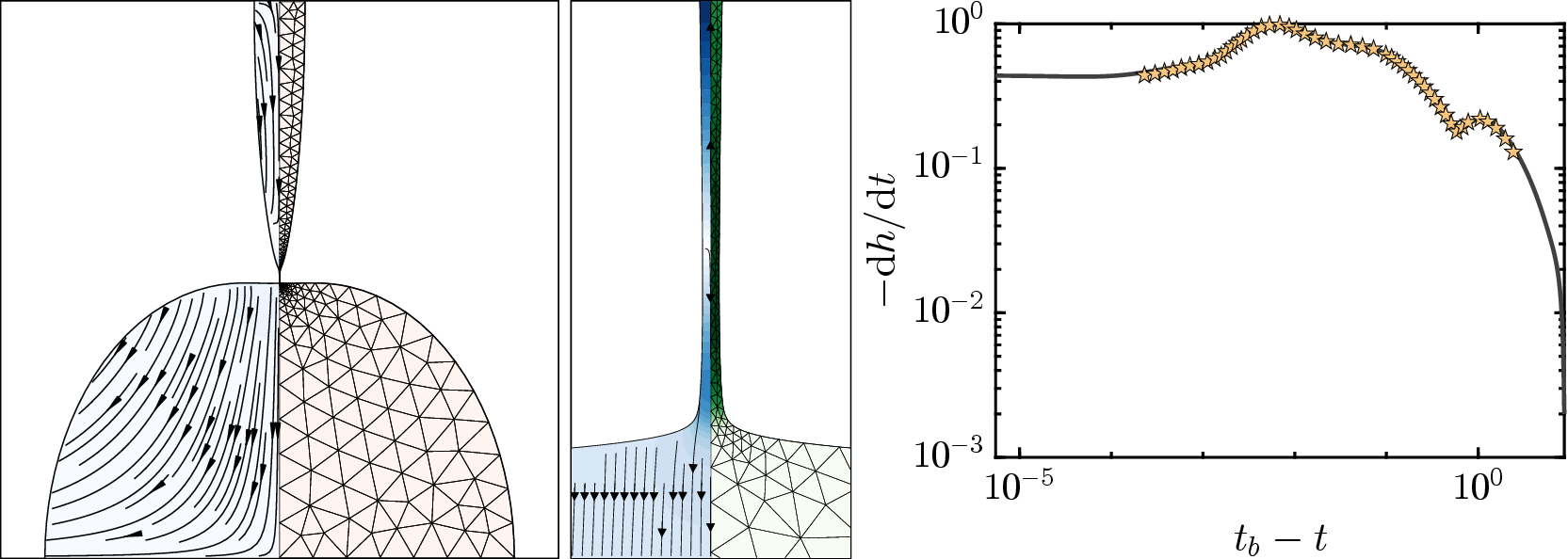
Fig. 6.6 Rayleigh-Plateau instability with advanced mesh size control and accurate boundary interpolation by \(\zeta\) coordinates : (left) Full view at the end of the simulation. (center) \(300\times\) zoom near on the position of minimum radius (right) Validation against literature (a higher mesh resolution used here).