10.3.1. Rayleigh-Benard convection in a cylindrical container
To illustrate the quite longish preface of this section by an example, let us consider a Rayleigh-Benard setting in a cylinder, which is heated from below and cooled from above, with no-slip boundary conditions at all walls. At some specific temperature difference (or better: Rayleigh number), convection will set in. We want to use the azimuthal stability framework to obtain the critical Rayleigh number \(\operatorname{Ra}\) as function of the aspect ratio \(\Gamma=R/H\) of the cylinder. We have to do it individually for each mode \(m\).
We start by the problem definition, analogous to the same case discussed in [16]:
from pyoomph import *
from pyoomph.equations.navier_stokes import * # Navier-Stokes for the flow
from pyoomph.equations.advection_diffusion import * # Advection-diffusion for the temperature
from pyoomph.utils.num_text_out import * # Output for the critical Rayleigh as function of the aspect ratio


class RBConvectionProblem(Problem):
    def __init__(self):
        super().__init__()
        # Aspect ratio, Rayleigh and Prandtl number with defaults
        self.Gamma = self.define_global_parameter(Gamma=1)
        self.Ra = self.define_global_parameter(Ra=1)
        self.Pr =self.define_global_parameter(Pr=1)

    def define_problem(self):
        # Axisymmetric coordinate system
        self.set_coordinate_system(axisymmetric)
        # Scale radial coordinate with aspect ratio parameter
        self.set_scaling(coordinate_x=self.Gamma)
        # Axisymmetric cross-section as mesh.
        # We use R=1 and H=1, but due to the radial scaling, we can modify the effective radius
        self+=RectangularQuadMesh(size=[1, 1], N=20)
By setting the spatial scale of "coordinate_x" in the axisymmetric coordinate system, we effectively scale the radial coordinate \(r\to\Gamma r\), so that we can modify the cylinder radius without changing the mesh at all. Of course, one should not go to extreme aspect ratios (\(\Gamma\ll 1\) or \(\Gamma \gg 1\)) by this, since the solution won’t be captured well then.
The rest starts trivially, just adding Navier-Stokes with body force given by the nondimensional temperature, which is solved by a corresponding advection-diffusion equation:
        RaPr=self.Ra*self.Pr # Shortcut for Ra*Pr
        # Equations: Navier-Stokes. We scale the pressure also with RaPr,
        # so that the hydrostatic pressure due to the bulk-force is independent on the value of Ra*Pr
        NS=NavierStokesEquations(mass_density=1, dynamic_viscosity=self.Pr,bulkforce=RaPr*var("T")*vector(0, 1), pressure_factor=RaPr)
        # Since u*n is set at all walls, we have a nullspace in the pressure
        # This offset is fixed by an integral constraint <p>=0
        # One could also set it via a DirichletBC(pressure=0) at e.g. a single corner,
        # but this yields problems in the azimuthal stability analysis then
        # The pressure integral constraint is automatically deactivated when m!=0, since <p>=0
        # holds automatically when p = p^(m)*exp(I*m*phi) for m!=0
        eqs = NS.with_pressure_integral_constraint(self,integral_value=0,set_zero_on_normal_mode_eigensolve=True)

        # And advection-diffusion for temperature
        eqs += AdvectionDiffusionEquations(fieldnames="T",diffusivity=1, space="C1")
With pressure_factor in the NavierStokesEquations, we scale the pressure with the product of the Rayleigh and Prandtl number. This product is entering the bulk force, i.e. the buoyancy. When scaling the pressure the same way, the stationary pressure field is independent of \(\operatorname{Ra}\operatorname{Pr}\). Thereby, one can solve the stationary conductive solution (mainly pressure and temperature field) for any Rayleigh number and change the Rayleigh number afterwards.
Furthermore, we have to fix the null space of the pressure, originating from the fact that only no-slip boundary conditions are used. Usually, we just pin e.g. a single corner to some pressure value. However, this is problematic, since it will also pin the corresponding eigenfunction value to zero there. A typical Dirichlet condition would just remove the pressure value at this corner from the unknowns and hence also from the pressure eigenfunction. Therefore, the volume average of the pressure is enforced to be zero instead. All pressure values remain unpinned and will have a degree of freedom in the eigenvector as well. However, when considering modes \(m\neq 0\), the average pressure of the eigenfunction will be automatically zero, since \(\exp(im\phi)\) averages to zero. In that case, we must deactivate this constraint to prevent overconstrainment. This is achieved by the keyword argument set_zero_on_normal_mode_eigensolve in the pressure null space removal with_pressure_integral_constraint().
The boundary conditions are straightforward:
        # Boundary conditions
        eqs += DirichletBC(T=0)@"bottom"
        eqs += DirichletBC(T=-1)@"top"
        # The NoSlipBC will actually also set velocity_phi=0 automatically
        eqs += NoSlipBC()@["top", "right", "bottom"]
        # Here, the magic happens regarding the m-dependent boundary conditions
        eqs += AxisymmetryBC()@"left"

        # Output
        eqs+=MeshFileOutput()

        # Add the system to the problem
        self+=eqs@"domain"
Note that the NoSlipBC will also set the \(\phi\)-component of the velocity to zero automatically. Also, note the AxisymmetryBC, which will set the correct boundary conditions for the azimuthal stability analysis, as outlined before. Also normal output is added, before the equation system is added to the problem. One last thing which has to be done when running the problem is to activate the azimuthal stability analysis. This is done by passing azimuthal_stability=True to the setup_for_stability_analysis() call. We also pass analytic_hessian=True, since we will use bifurcation tracking later on, which requires the Hessian to locate the bifurcation accurately:
        # Magic function: It will perform all necessary adjustments, i.e.
        #   -expand fields and test functions with exp(i*m*phi)
        #   -consider phi-components in vector fields, i.e. here velocity
        #   -incorporate phi-derivatives in grad and div
        #   -generate the base residual, Jacobian, mass matrix and Hessian, but also
        #    the corresponding versions for the azimuthal mode m!=0
        problem.setup_for_stability_analysis(azimuthal_stability=True,analytic_hessian=True)
The stationary conductive base state (\(u=0\), linear temperature profile, hydrostatic pressure) does not depend on the velocity at all. We therefore restrict the very first solve to the pressure and temperature degrees of freedom only, using select_dofs() in a with block:
        # Solve once to get the right pressure and temperature field. Velocity can stay zero here
        with problem.select_dofs() as dofs:
            dofs.unselect("domain/velocity_x","domain/velocity_y")
            problem.solve()
With the base state at hand, we loop over the azimuthal modes \(m=0,1,2,3\) we are interested in. For each mode, we start at a small aspect ratio \(\Gamma=0.5\) and a guess \(\operatorname{Ra}=10\), which is certainly stable. Since the conductive base state does not depend on \(\operatorname{Ra}\) at all, we do not have to solve the (unchanged) stationary problem again for each trial value of \(\operatorname{Ra}\); we only have to recompute the eigenvalues. This is exactly what find_bifurcation_via_eigenvalues() does: called as a generator with do_solve=False, it bisects on \(\operatorname{Ra}\) (with initial step initstep=200) until the largest of the neigen requested eigenvalues (for the azimuthal mode azimuthal_m=m) has a real part closer to zero than epsilon, yielding the current parameter and eigenvalue at each step:
        # Iterate over all desired modes m
        for m in [0,1,2,3]:
            problem.Gamma.value=0.5 # Start at some aspect ratio
            # Find a good guess for the critical Ra by eigenvalue bisection
            problem.Ra.value=10
            # We increase by steps of 200, but we don't have to solve the system, since the stationary solution is independent of Ra
            # we also pass the mode we want to solve for
            for currentRa,currentEigen in problem.find_bifurcation_via_eigenvalues("Ra",initstep=200,do_solve=False,neigen=4,azimuthal_m=m,epsilon=1e-2):
                print("Currently at Ra=",currentRa,"with eigenvalue",currentEigen)
Once we have a good guess for the critical Rayleigh number, we activate the bifurcation tracking via activate_bifurcation_tracking(), augmenting the system so that \(\operatorname{Ra}\) itself becomes an unknown that is solved for together with the critical eigenvector. For the axisymmetric mode \(m=0\), the bifurcation is a genuine pitchfork (as the base state still has the full rotational symmetry); for \(m\neq 0\), real and imaginary parts of the perturbation are coupled, so all such bifurcations are treated uniformly as "azimuthal". We then solve the augmented system to land exactly on the bifurcation and write the first row, \((\Gamma,\operatorname{Ra}_\text{c})\), to a text file dedicated to this mode:
            # Activate the bifurcation tracking. For mode m=0, we can have fold, pitchfork, etc.
            # For azimuthal modes m!=0, this distinguishment is not easily possible, since everything is complex anymways
            problem.activate_bifurcation_tracking("Ra",bifurcation_type="pitchfork" if m==0 else "azimuthal")

            # Find a solution at the cricical Ra and write output
            problem.solve()
            problem.output_at_increased_time()
            txtout = NumericalTextOutputFile(problem.get_output_directory(f"curve_m_{m}.txt"))
            txtout.header("Gamma", "Ra")
            txtout.add_row(problem.Gamma.value,problem.Ra.value)
Finally, we trace out the critical curve \(\operatorname{Ra}_\text{c}(\Gamma)\) up to \(\Gamma=3\) by arclength_continuation() in the aspect ratio \(\Gamma\), writing a row to the output file at each step. Since the bifurcation-tracking augmented system is solved exactly at every step (i.e. the eigenvalue stays at zero by construction), the notion of “how much the solution has changed” that arclength_continuation() uses to propose the next step size is not meaningful here; we therefore call reset_arc_length_parameters() after each step, so that the full max_ds is always tried again. Once the sweep for the current mode is done, the bifurcation tracking is deactivated again before moving on to the next mode \(m\):
            # Arclength continuation in the aspect ratio
            ds_max = 0.05
            ds=ds_max

            while problem.get_global_parameter("Gamma").value < 3.0:
                ds = problem.arclength_continuation("Gamma", ds,max_ds=ds_max)
                # Resetting the arclength parameters. Since the stationary solution does not change at all, this is beneficial.
                # Arclength continuation otherwise monitors how the solution changes, but it does not at all...
                problem.reset_arc_length_parameters()
                txtout.add_row(problem.Gamma.value,problem.Ra.value)

            # Deactivate for the next loop
            problem.deactivate_bifurcation_tracking()
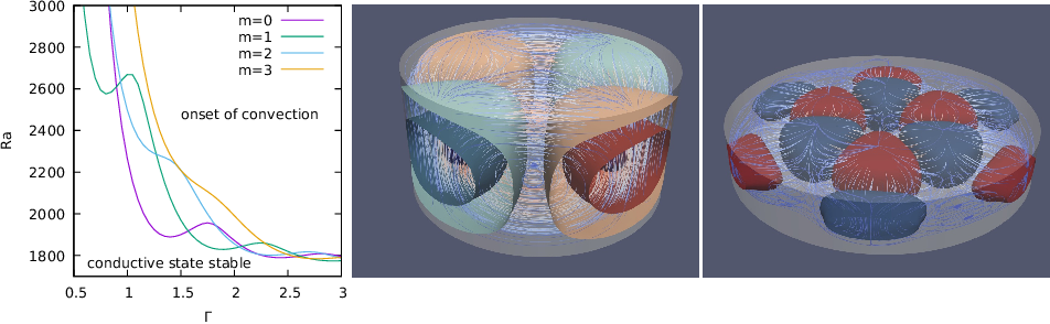
Fig. 10.4 Critical Rayleigh number for the onset of convection as function of the aspect ratio \(\Gamma\) and the critical eigenfunction for aspect ratio \(\Gamma=1\) and azimuthal mode \(m=2\) and \(\Gamma=m=3\), respectively.